Similarity Transformation and Orthogonal Transformation

SIMILARITY TRANSFORMATION AND ORTHOGONAL TRANSFORMATION

1. Similar matrices

Definition 1.4.1 Let A and B be square matrices of order n. A is said to be similar to B if there exists a non-singular matrix P of order n such that

A = P-1BP                  (1)

The transformation (1) which transforms B into A is called a similarity transformation. The matrix P is called a similarity matrix.

Note 

We shall now see that if A is similar to B then B is similar to A.

A = P-1BP ⇒ PA P-1 = B

 (Premultiplying by P and postmultiplying by P-1)

The relation (2) means B is similar to A. Thus, if A is similar to B, then B is similar to A. Hence we simply say similar matrices.

An important property of similarity transformations is that they preserve eigen values, which is proved in the next theorem.

Theorem 1. Similar matrices have the same eigen values.

Proof Let A and B be two similar matrices of order n.

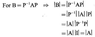
Then B = P-1 AP, by definition.

⸫ the characteristic polynomial of B is │B – λI│

⸫ A and B have the same characteristic polynomial and hence have the same characteristic equation. So A and B have the same eigen values.

Note Similar matrices A and B have the same determinant value i.e., |A| = |B|.

2. Diagonalisation of a square matrix

Definition 1.4.2 A square matrix A is said to be diagonalisable if there exists a non-singular matrix P such that P-1 AP = D, where D is a diagonal matrix. The matrix P is called a model matrix of A.

The next theorem provides us with a method of diagonalisation.

Theorem 1.4.2 If A is a square matrix of order n, having n linearly independent eigen vectors and M is the matrix whose columns are the eigen vectors of A, then M-1 AM = D, where D is the diagonal matrix whose diagonal elements are the eigen values of A.

Proof 

Let X1, X2,…, Xn be n linearly independent eigen vectors of A corresponding to the eigen values λ1, λ2, …., λ3 of A.

M-1AM = D

The matrix M which diagonalises A is called the model matrix of A and the resulting diagonal matrix D whose elements are eigen values of A is called the spectral matrix of A.

3. Computation of powers of a square matrix

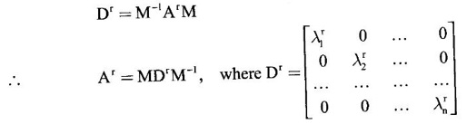
Diagonalisation of a square matrix A is very useful to find powers of A, say A'. By the theorem 1.4.2,

D = M-1AM

D2 = (M-1AM) (M-1AM)

= M-1A(MM-1)AM

= M-1AIAM = M-1A2M

Similarly,

D3 = D2D

= (M-1A2M) (M-1AM)

= M-1A2(MM-1)AM

D3 = M-1A2IAM = M-1A3M

Proceeding in this way, we can find

Note

(1) If the eigen values λ1, λ2, …., λn of A are different then the corresponding eigen vectors X1, X2, …, Xn are linearly independent by theorem 1.2.1 (2). So A can be diagonalised.

(2) Even if 2 or more eigen values are equal, if we can find independent eigen vectors corresponding to them (see worked example 6), then A can be diagonalised.

Thus independence of eigen vectors is the condition for diagonalisation.

Working rule to diagonalise a n × n matrix A by similarity transformation:

Step 1: Find the eigen values λ1, λ2, …., λn

Step 2: Find linearly independent eigen vectors X1, X2, …, Xn

Step 3: Form the modal matrix M = [X1, X2, …, Xn]

Step 4: Find M-1 and AM 

Step 5: Compute M-1AM = D =

4. Orthogonal matrix

Definition 1.4.3 A real square matrix A is said to be orthogonal if AAT = ATA = I, where I is the unit matrix of the same order as A.

From this definition it is clear that AT = A-1. So an orthogonal matrix is also defined as below.

Definition 1.4.4 A real square matrix A is orthogonal if AT = A-1.

Example 1

Prove that A = 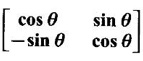is orthogonal.

Solution

⸫    A is orthogonal.

Properties of orthogonal matrix

1. If A is orthogonal, then AT is orthogonal.

Proof Given A is orthogonal.

⸫ AAT = ATA = I

Reversing the roles of A and AT, we see ATA = AAT = I

⇒  AT is orthogonal.

Note Since AT = A-1, it follows A-1 is orthogonal.

2. If A is an orthogonal matrix, then │A│= ±1.

Proof 

Given A is orthogonal. Then AAT = 1

⇒  |AAT| = 1

⇒ |A||AT| = 1

But we know

|AT| = |A|

⸫ |A||A| = 1

⇒  |A|2 = 1⇒ |A| = ±1

3. If λ is an eigen value of an orthogonal matrix A, then 1/ λ is also an eigen value of A.

Proof 

Given A is orthogonal and λ is an eigen value of A.

Then AT = A-1. By property (4) of eigen values,

1/ λ is an eigen value of A-1 and so an eigen value of AT.

By property (1), A and AT have same eigen values.

⸫ 1/ λ is an eigen of A and hence λ, 1/ λ are eigen values of orthogonal matrix A.

4. If A and B are orthogonal matrices, then AB is orthogonal.

Proof 

Given A and B are orthogonal matrices.

⸫ AT = A-1and BT = B-1

Now (AB)T = BT AT

= B-1A-1

= (AB)-1

AB is orthogonal.

5. Eigen values of an orthogonal matrix are of magnitude 1.

Proof 

Let A be an orthogonal matrix and let λ be an eigen value of A.

Then AX = λX, where X ≠ 0 (1)

Multiplying (2) and (1) we get

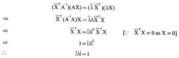
This is true for all eigen values of A.

Hence eigen values of A are of absolute value 1.

5. Symmetric matrix

Definition 1.4.5 A real square matrix A is said to be symmetric if AT = A.

Note that the elements equidistant from the main diagonal are same.

Properties of symmetric matrices

1. Eigen values of a symmetric matrix are real.

Proof 

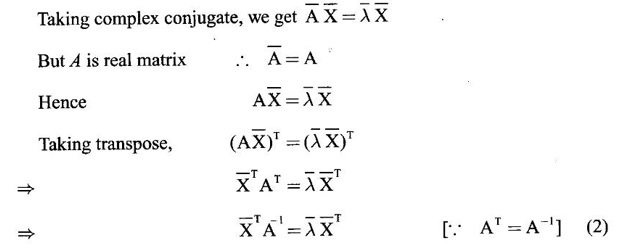
Let A be a symmetric matrix of order n and λ be an eigen value of A.

Then there exists X ≠ 0 such that AX = λX     (1)

Taking complex conjugate,

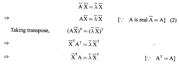
Post multiplying by X,

⸫ λ is real. This is true for all eigen values.

⸫ eigen values of a symmetric matrix are real.

2. Eigen vectors corresponding to different eigen values of a symmetric matrix are orthogonal vectors.

Proof 

Let A be a symmetric matrix of order n.

⸫  AT = A.

Let λ1, λ2 be two different eigen values of A. 

Then λ1, λ2 are real, by property (1).

⸫ there exist X1 ≠ 0, X2 ≠ 0 such that

Since λ1 ≠ λ2, λ1 - λ2 ≠ 0,      ⸫ X1TX2 = 0

⇒ X1 and X2 are orthogonal.

Remark If X1 = (a1, b1, c1) and X2 = (a2, b2, c2) be two 3-dimensional vectors, they are orthogonal if their dot product is 0⇒ a1a2 + b1b2 + c1c2 = 0

If we treat them as column matrices, then the matrix 

product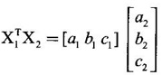

= a1a2 + b1b2 + c1c2

So X1 and X2 are orthogonal if X1TX2 = 0 or X2TX1 = 0.

Thus we can treat column matrices as vectors and verify dot product = 0.

2. The unit vector in X1 is and it is called a normalized vector.

Note 

For any square matrix eigen vectors corresponding to different eigen values are linearly independent, but for a symmetric matrix, they are orthogonal, pairwise.

6. Diagonalisation by orthogonal transformation or orthogonal reduction

Definition 1.4.6 A square matrix A is said to be orthogonally diagonalisable if there exists an orthogonal matrix N such that

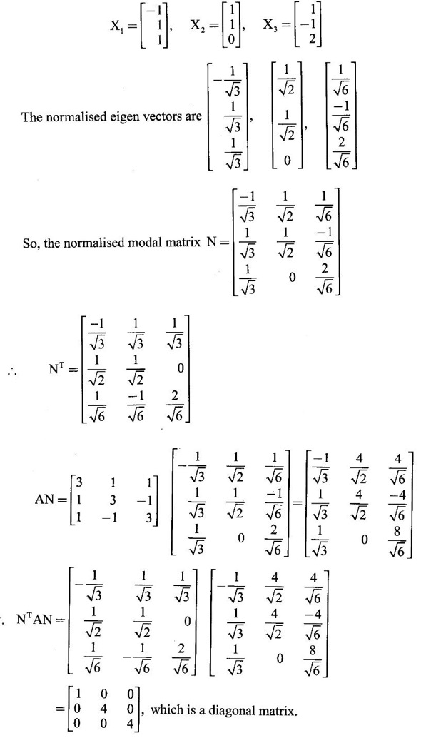
N-1 AN = D ⇒ NT AN = D   [⸪ NT = N-1]

This transformation which transforms A into D is called an orthogonal transformation or orthogonal reduction.

The next theorem gives a method of orthogonal reduction.

Theorem 1.4.3 Let A be a symmetric matrix of order n. Let X1, X2,…, Xn eigen vectors of A which are pairwise orthogonal. Let N be the matrix formed with the normalised eigen vectors of A as columns. Then N is an orthogonal matrix such that N-1 AN = D ⇒ NT AN = D.

N is called normalised model matrix of A or normal modal matrix of A.

Working rule for orthogonal reduction of a n × n symmetric matrix.

Step 1: Find the eigen values λ1, λ2,..., λn

Step 2: Find the eigen vectors X1, X2,..., Xn which are pairwise orthogonal.

Step 3: Form the normalised modal matrix N with the normalised eigen vectors

as columns.

Step 4: Find NT and AN.

Step 5: Compute NTAN = D =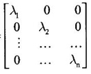

WORKED EXAMPLES

Example 1

Diagonalise the matrix A = 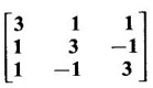by means of an orthogonal transformation.

Solution

A is a symmetric matrix. The characteristic equation of A is |A- λI| = 0

⇒ λ3 - S1λ2 + S2λ – S3 = 0

where

S1 = 3 + 3 + 3 = 9

⸫ the eigen values are λ = 1, 4, 4.

To find eigen vectors:

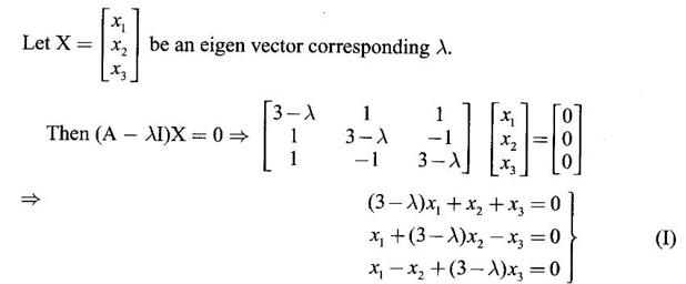
Case (i) If λ = 1 then equations (I) become

2x1 + x2 + x3 = 0

x1 + 2x2 - x3 = 0

x1 − x2 + 2x3 = 0

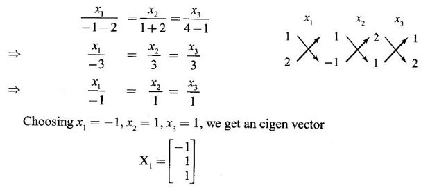
Choosing the first two equations, we have

Case (ii) If λ = 4, then the equations (I) become

-x1 + x2 + x3 = 0 ⇒ x1 - x2 - x3 = 0

x1 - x2 - x3 = 0

x1 − x2 - x3 = 0

We get only one equation x1 − x2 - x3 = 0        (1)

To solve for x1, x2, x3, we can assign arbitrary values for two of the variables and we shall find 2 orthogonal vectors.

Put x3 = 0, x2 = 1, then x1 = 1, we get an eigen vector

Let X3 = be ⊥ to X2. Then a + b = 0 ⇒ b = -a and X3 should satisfy (1) 

⸫ a – b – c = 0

Choosing a = 1, we get b = -1 and c = 2

Thus the eigen values are λ = 1, 4, 4, and the corresponding eigen vector are

Example 2

Diagonalise the symmetric matrix by an orthogonal transformation.

Solution

S3 = |A| = 2(1 – 4) −1(1 – 2) − (−2 + 1)

= -6 + 1 + 1 = -4

⸫ the characteristic equation is λ3 - 4 λ2 – λ + 4 = 0

By trial λ = 1 is a root.

Other roots are given by λ2 - 3 λ – 4 = 0

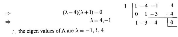
⸫ the eigen values of A are λ = −1, 1, 4

To find eigen vectors:

Let X = be an eigen vector corresponding to the eigen value λ.

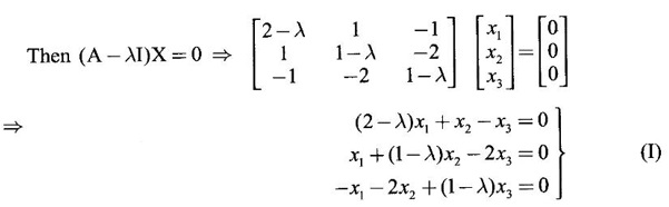
Case (i) If λ = -1, then the equations (I) become

3x1 + x2 - x3 = 0

x1 + 2x2 - 2x3 = 0

-x1 − 2x2 + 2x3 = 0 ⇒ x1 + 2x2 - 2x3 = 0

From the first two equations we get

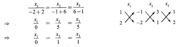
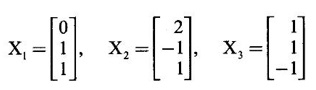
Choosing x1 = 0, x2 = 1, x3 = 1, we get an eigen vector,

Case (ii) If λ = 1, the equations (I) become

x1 + x2 - x3 = 0

x1 + 0x2 - 2x3 = 0

-x1 − 2x2 + 0x3 = 0 

From the first two equations, we get

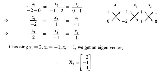
Case (iii) If λ = 4, the equations (I) become

-2x1 + x2 - x3 = 0

x1 - 3x2 - 2x3 = 0

-x1 − 2x2 - 3x3 = 0 

From the first and second equations, we get

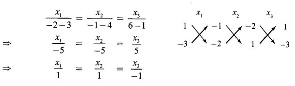
Choosing vector x1 = 1, x2 = 1, x3 = -1, we get an eigen vector

Thus the eigen values of A are −1, 1, 4 and the corresponding eigen vectors are

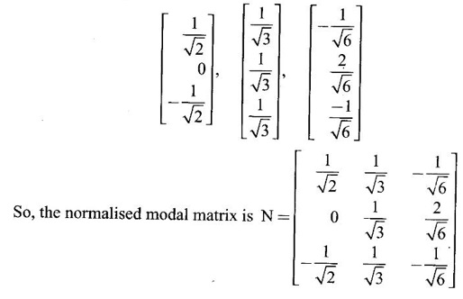
Since A is symmetric, the eigen vectors are pairwise orthogonal.

The normalised eigen vectors are

Example 3

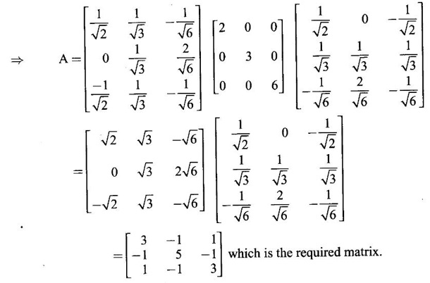
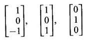
The eigen vectors of a 3 × 3 real symmetric matrix A corresponding to the eigen values 2, 3, 6 are [1, 0, −1]T, [1, 1, 1]T, [−1, 2, -1]T respectively, find the matrix A.

Solution

Given A is symmetric and the eigen values are different.

So, the eigen vectors are orthogonal pairwise.

The normalised eigen vectors are

Then by orthogonal reduction theorem 1.4.3

NTAN = D = 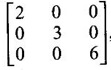, since 2, 3, 6 are the eigen values.

But NT = N-1

⸫ N-1AN = D ⇒ A = ND N-1 = NDNT

Example 4

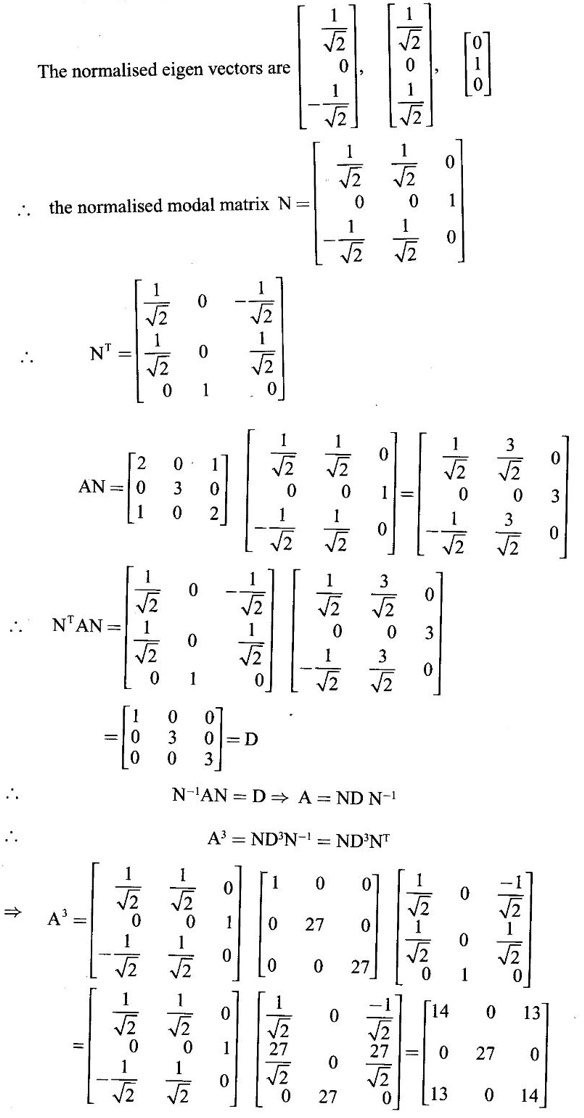
Diagonalise the matrix A = Hence find A3.

Solution

Given A = 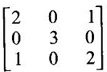which is a symmetric matrix.

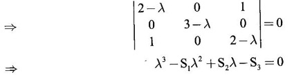
So, we shall diagonalise by orthogonal transformation. The characteristic equation of A is |A – λI| = 0

where S1 = 2 + 3 + 2 = 7

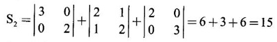
S3 = |A| = 2(6) − 0 +1(−3) = 12 − 3 = 9

⸫ the characteristic equation is λ3 − 7 λ2 + 15 λ – 9 = 0

By trial λ = 1 is a root.

To find eigen vectors:

Let X = be an eigen vector corresponding to eigen value λ.

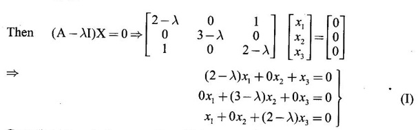
Case (i) If λ = 1, then equations (I) become

x1 + x3 = 0 ⇒ x3 = −x1

2x2 = 0 ⇒ x2 = 0

x1 + x2 = 0

Choose x1 = 1 ⸫ x3 = -1

⸫ an eigen vector is

Case (ii) If λ = 3, then equations (I) become

and            x2 can take any value

Choosing x1 = 1, we get x3 = 1 and choose x3 = 0

⸫ an eigen vector is     

We shall now choose X3 = orthogonal to X2

⸫ dot product = 0 ⇒ a + c = 0 and X3 should satisfy equations (2)

a - c = 0 and 0b = 0

Solving, we get a = c = 0 and choose b = 1

Thus the eigen values are 1, 3, 3 and the corresponding eigen vectors are

Clearly they are pairwise orthogonal vectors.

Example 5

Reduce the matrix 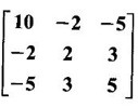to diagonal form.

Solution

Let A =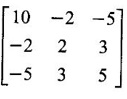

The characteristic equation is |A - λI| = 0.

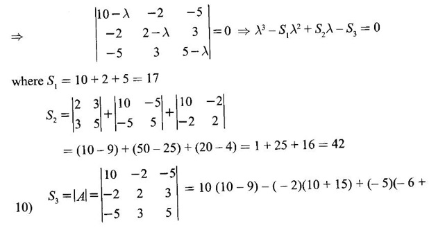
= 10 + 10 – 20 = 0

⸫ the characteristic equation is λ3 - 17 λ2 + 42λ = 0

⇒ λ (λ2 – 17 λ + 42) = 0

⇒ λ (λ − 3) (λ - 4) = 0 ⇒ λ = 0, 3, 14.

To find eigen vectors:

Let X = be an eigen vector corresponding to eigen value λ

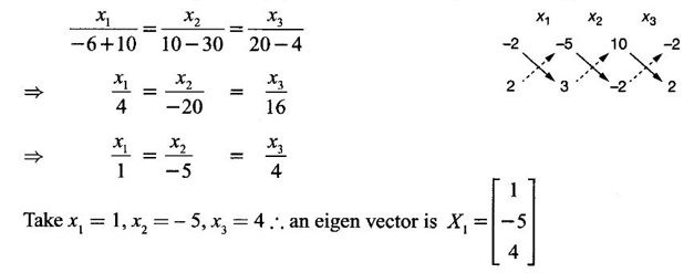
Case (i) If λ = 0, then (I) ⇒ 10x1 -2x2 - 5x3 = 0

-2x1 + 2x2 + 3x3 = 0

-5x1 + 3x2 + 5x2 = 0

From the first two equations, by rule of cross multiplication we get

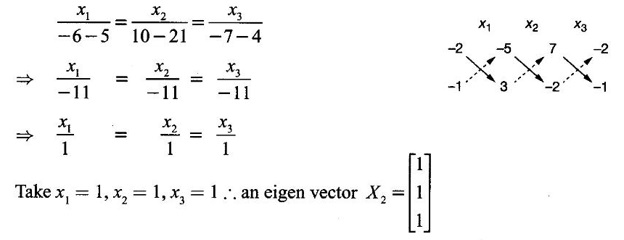
Case (ii) If λ = 3 then (I) ⇒ 7x1 -2x2 - 5x3 = 0

-2x1 - x2 + 3x3 = 0

-5x1 + 3x2 + 2x3 = 0

From the first two equation, by rule of cross multiplication, we get

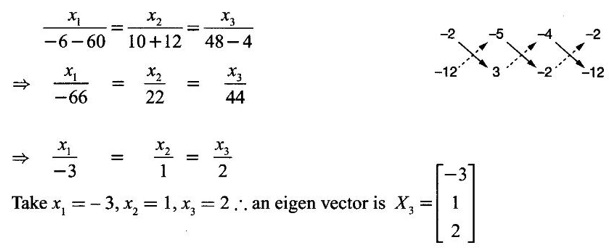
Case (iii) If λ = 14,  then (I) ⇒ -4x1 -2x2 - 5x3 = 0

-2x1 - 12x2 + 3x3 = 0

-5x1 + 3x2 - 9x3 = 0

From the first two equations, by rule of cross multiplication, we get

The matrix is symmetric and the eigen values are district and so the eigen vectors will be orthogonal

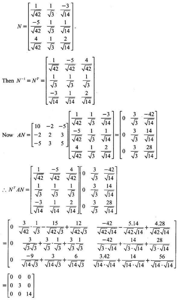
The normalized eigen vectors are

So, the normalized modal matrix is