Transforms and Partial Differential Equations: Unit III: Applications of Partial Differential Equations
One dimensional equation of heat conduction
Solved Example Problems
Consider a homogeneous bar of cross sectional area A. Take the origin O at one end of the bar and the positive x axis along the direction of heat flow.
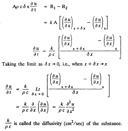
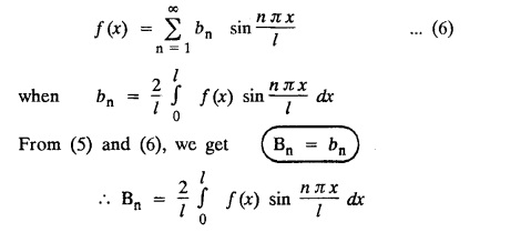
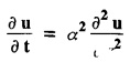
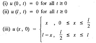
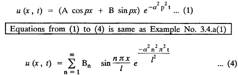
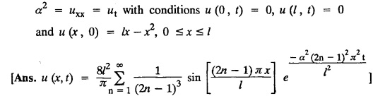
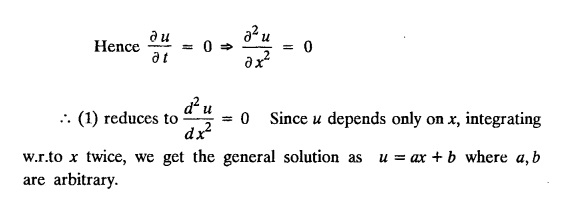
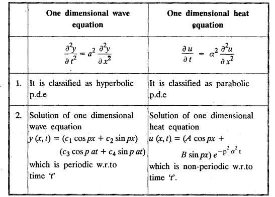
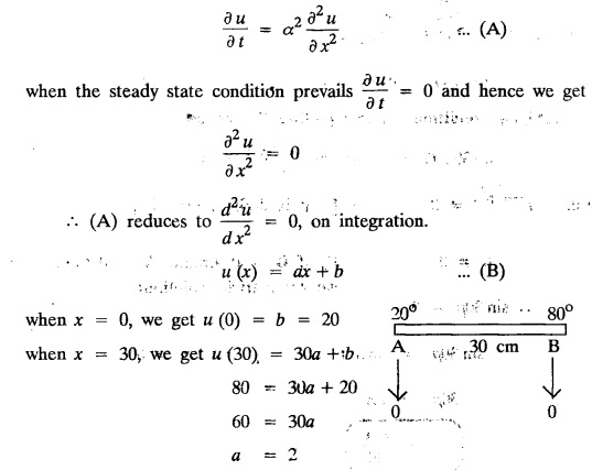
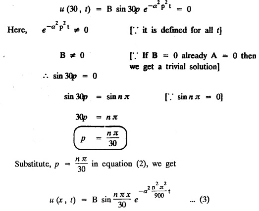
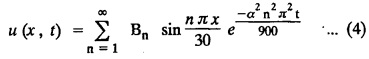
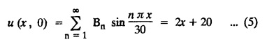
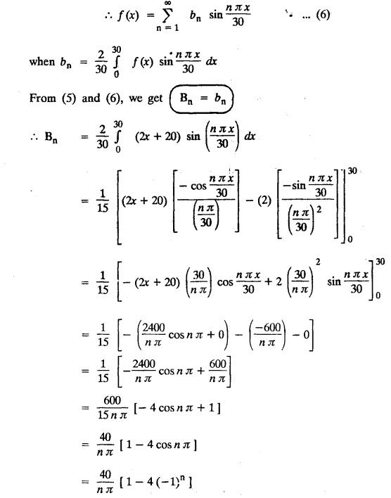
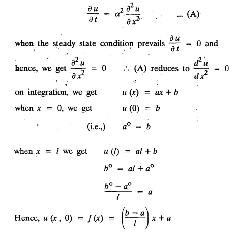
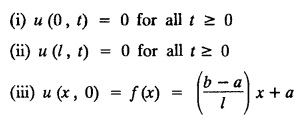
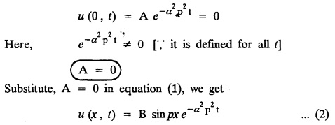
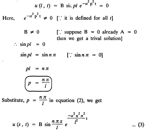
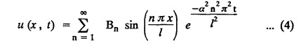
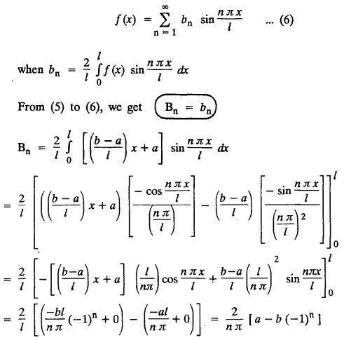
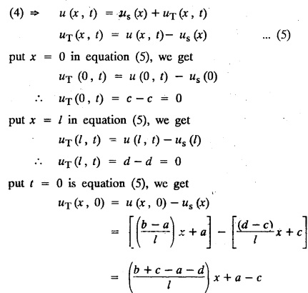
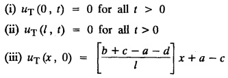
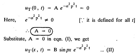
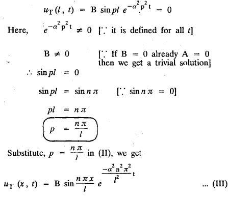
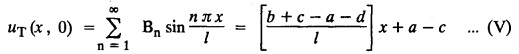
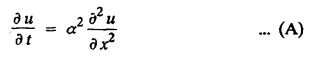
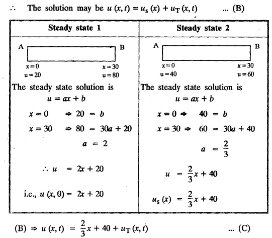
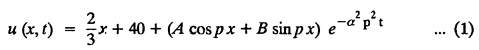
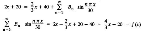
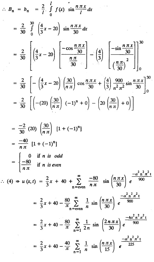
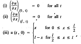
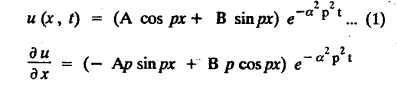
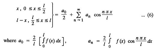
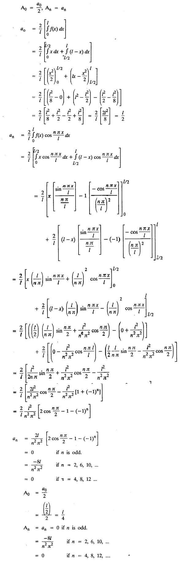
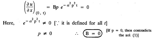
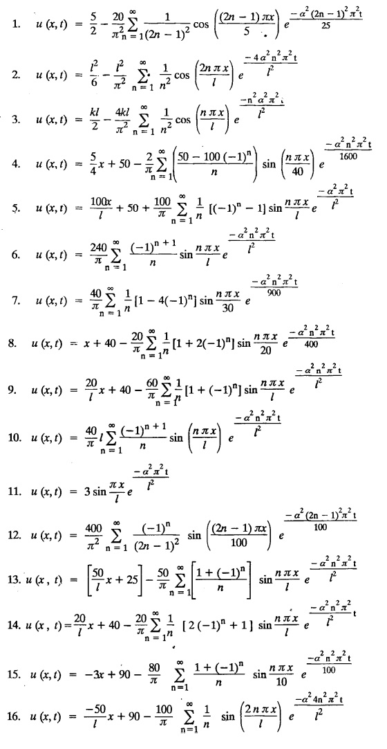
ONE DIMENSIONAL EQUATION OF HEAT CONDUCTION Consider a homogeneous bar of cross sectional area A. Take the origin O at one end of the bar and the positive x axis along the direction of heat flow. Let PQ be an element of length Ax and u (x, t), u(x + Δx, t) be the temperatures at time t at the ends P and Q respectively. Example 3.4.1: What are the assumptions made while deriving one dimensional heat equation? Solution: We assume the following experimental laws. 1. Heat flows from higher to lower temperature. 2. The amount of heat required to produce a given temperature change in a body is proportional to the mass of the body and to the temperature change. This constant of proportionality is known as the specific heat of the conducting material. 3. The rate at which heat flows across any area is proportional to the area and to the temperature gradient normal to the curve. This constant of proportionality is known as the thermal conductivity (k) of the material. It is known as Fourier's law of heat conduction. Example 3.4.2 : State Fourier's law of heat conduction. The rate at which heat flows across any area is proportional to the area and to the temperature gradient normal to the curve. This constant of proportionality is known as the thermal conductivity (k) of the material. It is known as Fourier's law of heat conduction. Let R1 be the rate at which heat enters the element PQ of the bar of cross sectional area A. Then Note: The rate at which heat flows across any area is jointly proportional to the area and to the temperature gradient normal to the area. Example 3.4.3 : Write the p.d.e. of the one dimensional heat flow. Solution : Example 3.4.4 : The p.d.e. of one dimensional heat equation is Solution: α2 is called the diffusivity of the material of the body through which heat flows. If ρ be the density, c the specific heat and k thermal conductivity of the material, we have the relation Example 3.4.5 : . Explain why α2 (instead of α) is used in the heat equation Solution : Since, the constants k,c,ρ are all positive We assume the following experimental laws to get the one dimensional heat flow equation. 1. Heat flows from higher to lower temperature. 2. The amount of heat required to produce a given temperature change in a body is proportional to the mass of the body and to the temperature change. This constant of proportionality is known as the specific heat of the conducting material. 3. The rate at which heat flows across any area is proportional to the area and to the temperature gradient normal to the curve. This constant of proportionality is known as the thermal conductivity (k) of the material. It is known as Fourier's law of heat conduction. Let us consider a homogeneous bar of uniform cross sectional area A. Assume that the sides of the bar are insulated so that the stream lines of heat flow are all parallel and perpendicular to the area. Take an end of the bar as the origin and the direction of heat flow as the positive x-axis. Let c be the specific heat and k the thermal conductivity of the material. Consider an element got between two parallel sections. BDEF and GHIJ at distances x and x + δx from the origin O, the sections being perpendicular to the x-axis. The mass of the element Αρδx Let u (x, t) be the temperature at a distance x at time t. By the second law, the rate of increase of heat in the element If R1 and R2 are respectively the rates of inflow, and outflow, for the sections x = x and x = x + δx, then the negative sign being due to the fact that heat flows from higher to lower temperature. Equating the rate of increase of heat from the two empirical laws, If we denote it by α2, the above equation takes the form X is a function of x alone and T is a function of 't' alone. Case (i) Let k be positive k = p2 The auxiliary equations are Thus the various possible solutions of the heat equation (1) are Example 3.4.6: How many boundary conditions are required to solve Solution: Three. Example 3.4.7: State one dimensional heat equation with the initial and boundary conditions. Solution: The one dimensional heat equation is where u (x, t) is the temperature at time t at a point of distance x from the left end of the rod. The boundary conditions are (i) u (0,t) = k1°C for all t ≥ 0 (ii) u (l,t) k2°C for all t ≥ 0 ( l being the length of the one dimensional rod) The initial condition is (iii) u (x, 0) = f(x), 0 < x < 1 Problems with zero boundary values (Temperature or temperature gradients) Example 3.4.a(1) : A rod of length l with insulated side is initially at a uniform temperature f(x). Its ends are suddenly cooled to 0°C and are kept at the temperature. Find the temperature function (x, t). (OR) Solve the equation Solution : The temperature function u (x, t) satisfies the one dimensional heat equation is From the given problem, we get the following boundary and initial conditions. Now, the suitable solution which satisfies our boundary conditions is given by Applying condition (i) in equation (1), we get Substitute, A = 0 in equation (1), we get Now, applying condition (ii) in equation (2), we get The most general solution is Applying condition (iii) in equation (4), we get 5 To find Bn expand ƒ (x) in a half-range Fourier sine series in the interval (0, l) Substitute, Bn value in equation (4), we get the general solution. Example 3.4.a(2) : Solve Solution : The temperature function u (x, t) satisfies the one dimensional heat equation is From the given problem, the boundary and initial conditions are Now, the suitable solution which satisfies our boundary conditions is given by Apply condition (iii) in equation (4), we get To find Bn expand the given f (x) in a half range Fourier sine series in the interval [0, l] Substitute, B value in equation (4), we get Example 3.4.a(3): A homogeneous rod of conducting material of length l has its ends kept at zero temperature. The temperature at the centre is T and falls uniformly to zero at the two ends. Find u (x, t). Solution: The temperature function u (x, t) satisfies the one dimensional heat equation is From the given problem we get the following boundary and initial conditions Since the temperature at the centre is T and falls uniformly to zero at the two ends, its distribution at t = 0 is as given in the figure. The equation of OB is The equation of BA is Now, the suitable solution which satisfies our boundary conditions is given by Applying condition (iii) in equation (4), we get To find Bn expand ƒ (x) in a half range Fourier sine series in the interval [0, l] From equations (5) and (6), we get Bn = bn Substitute Bn value in equation (4), we get 1. A rod l cm long with insulated lateral surface is initially at temperature uo, at an inner point distance x cm from one end. If both ends are kept at zero temperature. Find the temperature function at any point of the rod at any time t. 2. Solve the boundary value problem : 3.4b. Steady state conditions and zero boundary conditions: Problems based on Steady state conditions and zero boundary conditions Example 3.4.b(1) What is meant by steady state condition in heat flow ? Solution : Steady state condition in heat flow means that the temperature at any point in the body does not vary with time. i.e., it is independent of t, the time. Example 3.4.b(2): In steady state conditions, derive the solution of one dimensional heat flow? Solution: The p.d.e. of unsteady one dimensional heat flow is In steady state condition, the temperature u depends only on x and not time t Example 3.4.b(3): What is the basic difference between the solution of one dimensional wave equation and one dimensional heat equation? Solution : Example 3.4.b(4) : Distinguish between steady and unsteady states in heat conduction problems. Solution : In unsteady state, the temperature at any point of the body depends on the position of the point and also the time t. In steady state, the temperature at any point depends only on the position of the point and is independent of the time t. Example 3.4.b(5) : A rod 30 cm long has its ends A and B kept at 20° and 80° respectively until steady state conditions prevail. The temperature at each end is then suddenly reduced to 0° C and kept so. Find the resulting temperature function u (x, t) taking x = 0 at A. Solution : The temperature function u (x, t) is the solution of the one dimensional heat equation Thus u (x, 0) = f(x) = 2x + 20 by (B) Hence, Boundary and initial conditions are Now, the suitable solution which satisfies our boundary conditions is given by Applying condition (i) in (1), we get Now, applying condition (ii) in equation (2), we get The most general solution is Applying condition (iii) in equation (4), we get To find Bn expand 2x + 20 in a half range Fourier sine series in the interval (0, 30) Substitute, the value of Bn in equation (4), we get Example 3.4.b(6) : An insulated rod of length l has its ends A and B kept at a° celsius and b° celsius respectively until steady state conditions prevail. The temperature at each end is suddenly reduced to zero degree celsius and kept so. Find the resulting temperature at any point of the rod taking the end A as origin. Solution: The temperature function u (x, t) is the solution of the one dimensional heat equation. The boundary and initial conditions are Now, the suitable solution which satisfies our boundary conditions is given by Applying condition (i) in equation (1), we get Applying condition (ii) in equation (2), we get The most general solution is Applying condition (iii) in eqn. (4), we get To find Bn expand ƒ (x) in a half range Fourier sine series in the interval (0, l) Substitute the value of Bn in equation (4), we get 3.4c. Steady state conditions and non-zero Boundary conditions Problems based on Steady state conditions and non-zero Boundary conditions Example 3.4.c(1): A rod of length l cm with insulated sides has its ends A and B kept at a° celsius and b° celsius respectivley until steady state conditions prevail. The temperature at A is then suddenly raised to c° celsius and that at B is lowered to d° celsius. Find the subsequent temperature distribution u (x, t). Solution: The equation to be solved is Applying condition (i) in equation (1), we get Applying condition (ii) in equation (1), we get From equation (2) and (3) it is not possible to find the constants A and B. Since, we have infinite number of values for A and B. Therefore in this case, we split the solution u (x, t) into two parts. uT (x, t) is a transient solution satisfying equation (4) which decreases as t increases. If u (x, t) is the subsequent temperature function the boundary and initial conditions are To find us (x) To find uT (x, t) ⸫ Given new boundary and initial conditions are Now, the suitable solution is Applying condition (i) in (I), we get Applying condition (ii) in (II), we get The most general solution is Now, applying conditions (iii) in (IV), we get To find Bn we expand ƒ (x) in a half range Fourier sine series Substitute, the value of Bn in IV, we get Example 3.4.c(2) : The ends A and B of a rod 30 cms long have their temperature kept at 20° C and the other at 80° C until steady state conditions prevail. The temperature of the end B is then suddenly reduced to 60° C and kept so while the end A is raised to 40° C. Find the temperature distribution in the rod after time t. Solution : The equation to be solved is Here, there are two steady states The boundary and initial conditions are Now, the suitable solution which satisfies our boundary conditions is given by Applying condition (i) in equation (1), we get Substitute, A = 0 in equation (1), we get Applying condition (ii) in equation (2), we get The most general solution is Applying condition (iii) in equation (4), we get To find Bn Expand f(x) in a Half-range Fourier sine series in the interval (0,l) 3.4d. Thermally insulated ends Problems based on Thermally insulated ends Example 3.4.d(1): Explain the term "Thermally insulated End's". Solution: If an end of heat conducting body is thermally insulated, it means that no heat passes through that section. Mathematically, the temperature gradient is zero at that point. Example 3.4.d(2) : Express the boundary conditions in respect of insulated ends of a bar of length a and also the initial temperature distribution. Solution : The boundary and initial conditions are Example 3.4.d(3) : Solve : Solution: The equation to be solved is From the given problem, we get the following boundary and initial conditions. Now, the suitable solution which satisfies our boundary conditions is given by Applying condition (i), we get The most general solution is Applying condition (iii) in (4), we get To find A0 and An expand ƒ (x) in a half range cosine series in (0, l). Equations from (5) and (6), we get Substitute the values of A0 and An is equation (4), we get Example 3.2.d(4): Solution : The equation to be solved is From the given problem, we get the following boundary and initial conditions. (i) ux (0, t) = 0 (ii) ux (π, t) = 0 (iii) u (x, 0) = sin x Now, the suitable solution which satisfies our boundary conditions is given by Applying condition (i), we get Substitute the value of B = 0 in equation (1), we get Applying condition (ii), we get The most general solution is EXERCISE 3.4 1. Solve the boundary value problem 4. A bar of 40 cm long has originally a temperature of 0° C along all its length. At t = 0, the temperature at the end x = 0 is raised to 50° C, while at the other end it is raised to 100° C. Determine the resulting temperature function. 5. A rod of length has its ends A and B kept at 0° C and 100° C until steady state conditions prevail. If the temperature of A is suddenly raised to 50° C and that of B is 150° C, find the temperature distribution at any point. 6. A rod of length / has its ends A and B kept at 0° C and 120° C respectively, until steady state condition prevail. If the temperature at B is reduced to 0o C and kept so, while that of A is maintained, find the temperature distribution of the rod. 7. A rod of 30 cm long has its ends A and B kept at 20° C and 80° C respectively until steady state conditions prevail. The temperature at each end is then suddenly reduced to 0° C and kept so, find the resulting temperature distribution function u (x, t) taking x = 0 at A. 8. The ends A and B of a rod of 20 m length have temperature 30° C and 80° C until steady state prevails. The temperature of the ends are then suddenly changed to 40° C and 60° C respectively. Find the temperature distribution of the rod. 9. The ends A and B of a rod of length I have their temperature kept at 10° C and 90° C until steady state conditions prevail. The temperature of the end A is suddenly raised to 40° C and kept so while the end B is reduced to 60° C. Find the temperature distribution in the rod for the subsequent time. 12. A homogeneous rod of conducting material of length 100 cm has its ends kept at zero temperature and the initial temperature distribution is Find the temperature u (x, t) at any time. 13. A rod of length has its ends A and B kept at 0°C and 100° C respectively, until steady state conditions prevail. The temperature at A is raised to 25° C while that at B is reduced to 75° C. Find the temperature u (x, t) at a distance x from A and at time t. 14. The ends A and B of a rod l c.m. long have their temperatures kept at 30° C and 80° C, until steady state conditions prevail. The temperature of the end B is suddenly reduced to 60°C and that of A is increased to 40°C. Find the temperature distribution in the rod after time t. 15. A bar 10 cm long with insulated sides, has its ends A and B kept at 50° C and 100°C respectively until steady state conditions prevail. The temperature at A is then suddenly raised to 90°C and at the same instant that at B is lowered to 60° C and maintained thereafter. Find the subsequent temperature distribution in the bar. 16. The ends A and B of a rod l cm long have the temperature 40°C and 90°C until steady state prevails. The temperature at A is suddenly raised to 90°C and at the same time that at B is lowered to 40°C. Find the temperature distribution in the rod at time t. Also show that the temperature at the mid point of the rod remains unaltered for all time, regardless of the material of the rod. ANSWERS 3.4§ "Temperature - gradient".

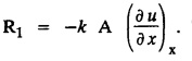 This is mathematical form of Fourier's law. We put a negative sign, as
  is negative. Heat flows from higher to lower temperature. As x increases, u decreases.
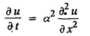
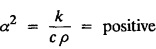
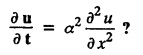
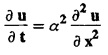 what is α2?
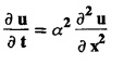

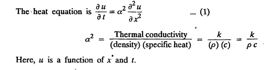
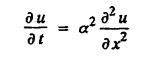
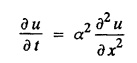
§ ONE DIMENSIONAL HEAT FLOW


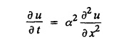
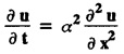
§ SOLUTION OF HEAT EQUATION
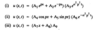
 So, assume that solution of (1) is of the form
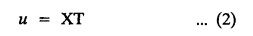


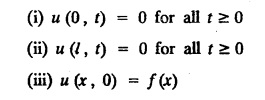
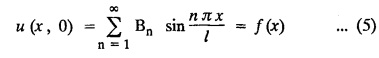
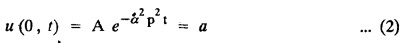
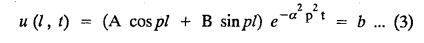
 subject to the conditions u (0, t)=0, u (l, t) = 0 and u(x, 0) = f(x).


 subject to the conditions


EXERCISE 3.4a


 subject to the conditions.


Transforms and Partial Differential Equations: Unit III: Applications of Partial Differential Equations : Tag: : Solved Example Problems - One dimensional equation of heat conduction
Related Topics
Related Subjects

Transforms and Partial Differential Equations
MA3351 3rd semester civil, Mechanical Dept | 2021 Regulation | 3rd Semester Mechanical Dept 2021 Regulation