Matrices and Calculus: Unit II: Differential Calculus
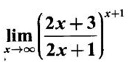
Limit of a Function
Definition, Theorem, Solved Example Problems | Differential Calculus
The essential idea of limit of a function is “nearness" to a point.
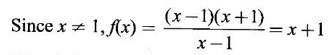
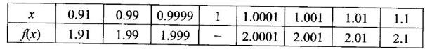
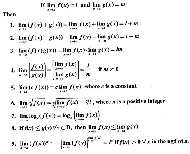
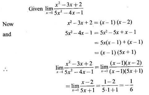
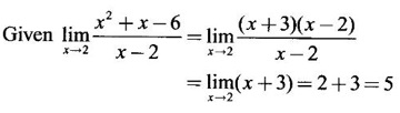
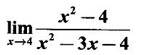
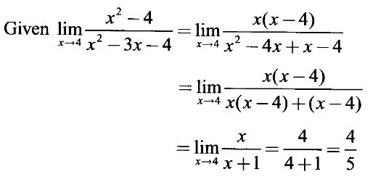
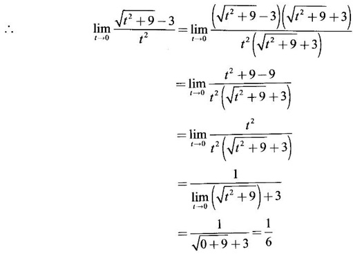
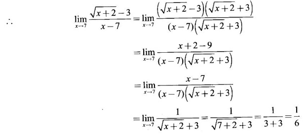
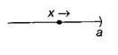
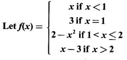
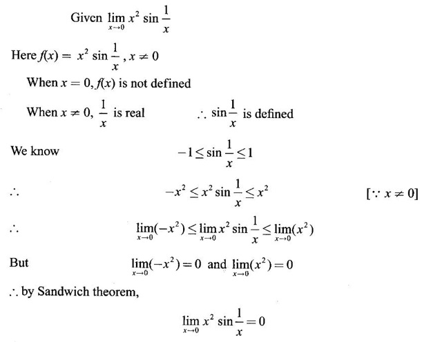
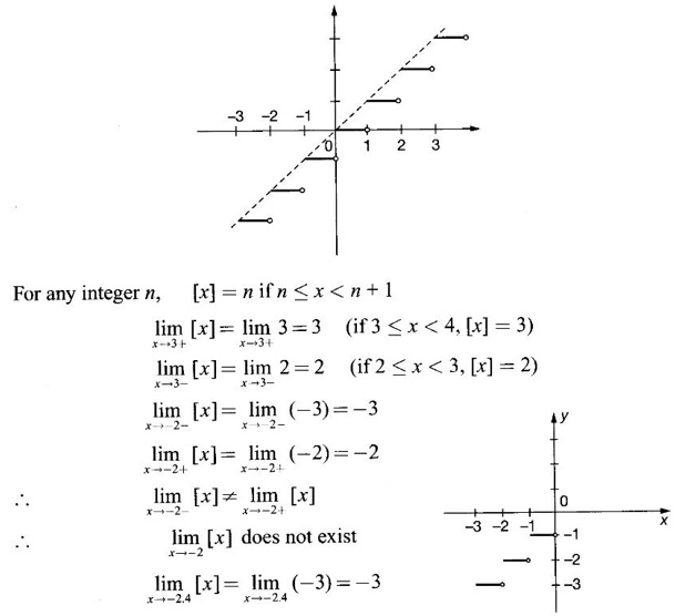
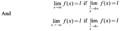
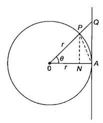
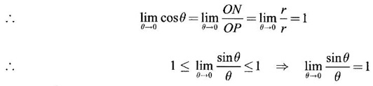
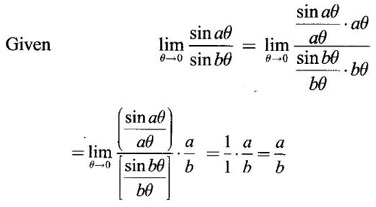
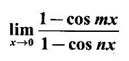
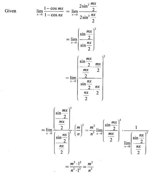
LIMIT OF A FUNCTION The essential idea of limit of a function is “nearness" to a point. Roughly, the limit process involves examining the behaviour of the function ƒ near a point a. The nearness is restricted to an open interval of the form (a - δ, a + δ), where δ is a small positive number. This open interval is called a neighborhood of a. Limiting behaviour occurs in a variety of practical problems. For example, Absolute zero, the temperature T at which all molecular activity ceases, can be approached but never actually attained. Similarly engineering profiling the ideal specification of a new engine are really dealing with limiting behaviours. To motivate mathematically, consider the function Suppose we want to know what happens if x approaches 1. We tabulate near 1 on the right side and left side of 1 in a neighborhood (1 − 0.1, 1 + 0.1) = (0.9, 1.1) x approaches 1 from left → ← x approaches 1 from right We find when x is close to 1 from the left or from the right, f(x) is close to 2 ⸫ f(x) approaches 2 as x approaches 1 from either side. Generalising this we now give an informal definition of limit. Definition 2.9 Limit Let f be a function defined in a neighborhood of a, except possibly at the point a. If f(x) is arbitrarily close to l for all x sufficiently close to a from either side, then we say that f(x) approaches l as x approaches a and we write lim f(x) = l This is read as "the limit of f(x) as x approaches a is l" Note: We shall now give the precise definition of limit. Definition 2.9(a) Precise definition of limit Let f be a function defined in a neighbourhood of a, except possibly at the point a. Then Note In this definition the modulus inequalities can be rewritten in terms of interval as stated as below It is illustrated in the graph. To evaluate limits the definition alone is not enough. The next theorem gives the basic properties of limit. Theorem 2.1 Note: If f(x) < g(x) ∀ x ∈ D, we cannot say Theorem 2.2 Sandwich theorem or the squeeze theorem As a consequence of the basic limits, we have the following standard limits Remark: Suppose Evaluate the following limits Example 1 Solution Example 2 Evaluate Solution Given Example 3 Evaluate Solution Given Example 4 Solution Example 5 Evaluate Solution Example 6 Solution Example 7 Solution Given Example 8 Solution Given Example 9 Solution Example 10 Evaluate Solution Example 11 Evaluate Solution Example 12 Evaluate Solution Example 13 Evaluate Solution Example 14 Solution Given Since denominator → 0 as t → 0, we cannot use quotient rule of limits. First we simplify by rationalizing the numerator. Multiply numerator and denominator by Example 15 Solution Given As x → 7, Denominator → 0 ⸫ first simplify by rationalizing the Numerator, Example 16 Solution ⸫ first simplify by rationalizing the Denominator, Example 17 Solution Given As x → 0, Denominator → 0 ⸫ first simplify by rationalizing the Numerator, Sometimes the limit of a function may not exist but only one side limit may exist i.e., either left side limit or right side limit may exist. Definition 2.10 Left-hand limit or left limit If the values f(x) of a function ƒ approach arbitrarily close to l for all x sufficiently close to a from the left of a (i.e, x < a), then the left-hand limit exists and is written as Similarly, if the values f(x) of ƒ approach arbitrarily close to l for all x sufficiently close to a from the right of a (i.e, x > a) then the right-hand limit exists and is written as For Example If f(x) = Solution The function is not defined at x = 0 but defined in the neighborhood of 0. ⸫ at x = 0, left-hand limit = -1 and right-hand limit = 1 The next theorem connects limit and one-sided limit Theorem 2.3 Note: By the theorem, in the above example Because Example 1 If f(x) = then determine whether Solution Since on the left side and right side of 4, ƒ is defined differently, we find one- sided limits. Left limit: Right limit: Example 2 Evaluate Solution Example 3 Find the limit if it exists? If the limit does not exist explain why? Solution Given limit is the left limit Example 4 Solution Example 5 (i) Evaluate the following (ii) Sketch the graph of ƒ Solution (ii) If x < 1, then the graph is y = x, which is a straight line bisecting the angle between the positive x and y axis. If x = 1, then the graph is a point (1, 3). If 1 < x ≤ 2, then the graph is y = 2 - x2 ⇒ x2 = 2 – y = - (y - 2) which is a parabola (of the form x2 = -4ay), with vertex (0, 2), and the axis is x = 0 i.e., the y-axis and downward If x > 2, then the graph is y = x - 3 which is a straight line Put x = 0, then y = -3 and put y = 0, then x = 3 ⸫ two points on it are (0, --3), (3, 0) We shall now draw the graph Example 6 Show that Solution Example 7 If f(x) = [x] is the greatest integer function, then find the limits if it exists. Solution Given f(x) = [x] With the real number set ℝ we add two symbols -∞ and +∞ or ∞ and get a larger set ℝ* = ℝ∪{-∞, ∞} ℝ* is called the extended real number system subject to the following rules (i) −∞ < x ∞ ∀ x ∈ ℝ i.e., any real number lies between these symbols. We also write ℝ = the open interval (-∞, ∞) (ii) For any real number x, x + ∞ = ∞, x - ∞ = - ∞ (iii) ∞ + ∞ = ∞, -∞ + (-∞) = -∞ (iv) For any real number, (v) If x > 0, x·∞ = ∞, x⋅(-∞) = -∞ If x < 0, x.∞ = -∞, x⋅(-∞) = ∞ (vi) ∞.∞ = ∞, -∞·∞ = -∞ = ∞·(-∞) (-∞)(-∞) = ∞ However, In our discussions whenever -∞ or ∞ is involved then we are discussing in ℝ* Consider the function In a neighborhood of 0, when we approach 0 from the right side 1/x is increasing indefinitely i.e., When we approach 0 from the left (i.e., through negative values) 1/x decreases indefinitely i.e., We describe these limiting behaviours by writing The graph of Definition 2.11 Infinite limits Let ƒ be a function defined in a neighbourhood of a, except possible at a. Definition 2.12 Vertical Asymptote The line x = a is called a vertical asymptote to the curve y = f(x) if For the curve y = 1/x, the line x = 0 or y-axis is a vertical asymptote because The word asymptote comes from the Greek word 'asymptotos' which means non intersecting. Definition 2.13 Horizontal asymptote A line y = b is a horizontal asymptote of the curve y = f(x) if either For the curve y = 1/x, the line y = 0 or x-axis is a horizontal asymptote because Note In the evaluation of limits of rational function and irrational functions involving polynomial as x → ± ∞, we manipulate the function so that the powers of x are transformed to powers of 1/x· This is done by pulling out the highest power of x in the numerator and denominator. Evaluate the following limits Example 1 Solution Second Method: Another method is by the transformation of the variable x Example 2 Solution Example 3 Solution Example 4 Solution Second Method: Example 5 Prove that Solution Theorem 2.4 Proof: Consider a circle with centre O and radius r. Let θ be a small angle in radian and let AOP = Draw PN ⊥ OA and the tangent at A meet OP produced at Q. From figure, we find that Area of ΔAOP < Area of sector AOP < Area of ΔAOQ Replacing θ by - θ, the in equality holds. So, the inequality holds for As θ → 0, P approaches along the arc of the circle to A and ON→OA = r In this formula θ is radian. Evaluate the following limits Example 1 Solution Example 2 Solution Example 3 Solution Example 4 Solution Example 5 Solution In limits with trigonometric functions if the variable x tends to a nonzero number, say Example 6 Solution Example 7 Solution Example 8 Solution Example 9 Solution Example 10 Solution Example 11 Solution Example 12 Solution Evaluate the following limits Example 13 Solution Example 14 Solution Example 15 Solution Example 16 Solution Example 17 Solution Example 18 Solution Evaluate the following limits

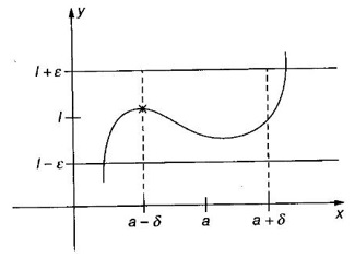
![]() f(x) = l means that for every ∈ > 0, there exists δ > 0 such that
f(x) = l means that for every ∈ > 0, there exists δ > 0 such that
 means that for every ∈ > 0, there exists a δ > 0 such that
 but we can only conclude


 exists, then
  need not exist.
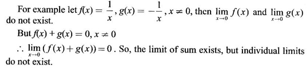
WORKED EXAMPLES


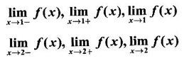
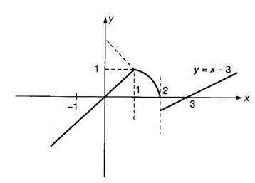
1. One-Sided Limits


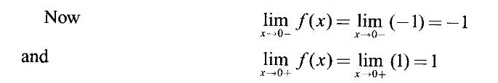

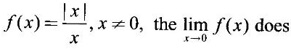 not exist.
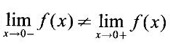
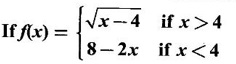
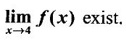
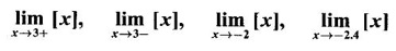
WORKED EXAMPLES

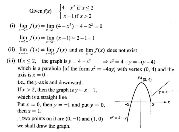
 8 − 2.4 = 0
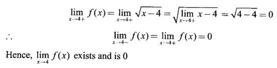


2. Extended Real Number System
 are indeterminates
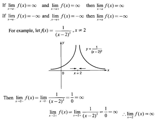
3. Infinite Limits


 and
and 
 ⇒ xy = 1, which is the rectangular hyperbola


WORKED EXAMPLES


4. Limits with Trigonometric Functions


![]() < θ < 0 also.
< θ < 0 also.
WORKED EXAMPLES


 then we convert it to tend to zero by putting


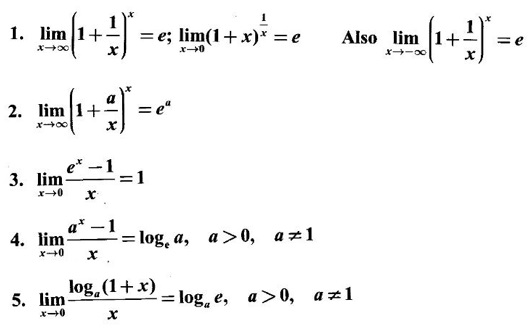
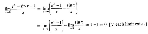
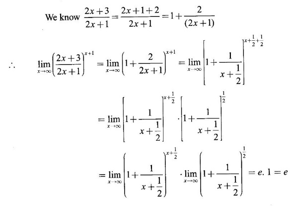
5. Limits with Exponential and Logarithmic Functions Standard Limits
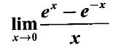
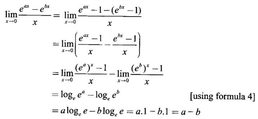
WORKED EXAMPLES


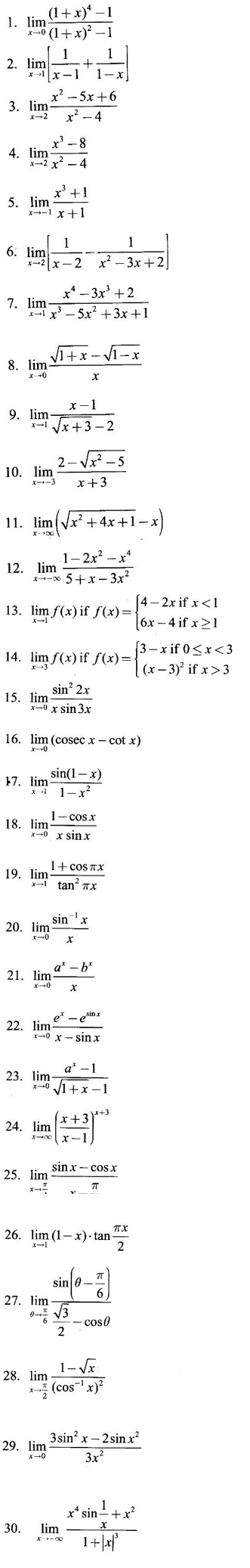
EXERCISE 2.3
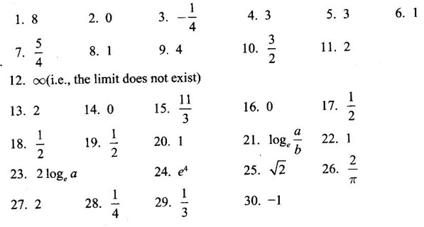
ANSWERS TO EXERCISE 2.3
Matrices and Calculus: Unit II: Differential Calculus : Tag: : Definition, Theorem, Solved Example Problems | Differential Calculus - Limit of a Function
Related Topics
Related Subjects
Matrices and Calculus
MA3151 1st semester | 2021 Regulation | 1st Semester Common to all Dept 2021 Regulation