Matrices and Calculus: Unit V: Multiple Integrals
Double Integration
Worked Examples, Exercise with Answers
Double integrals occur in many practical problems in science and engineering.
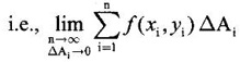
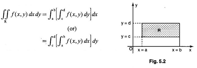
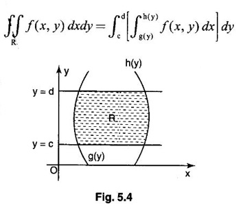
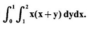
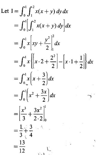
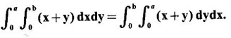
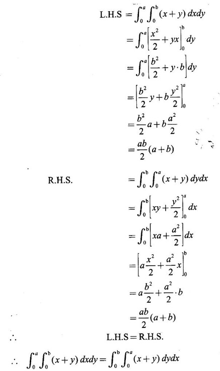
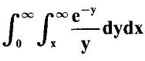
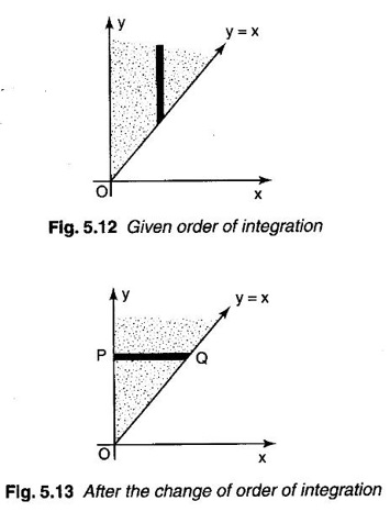
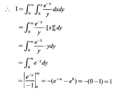
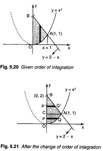
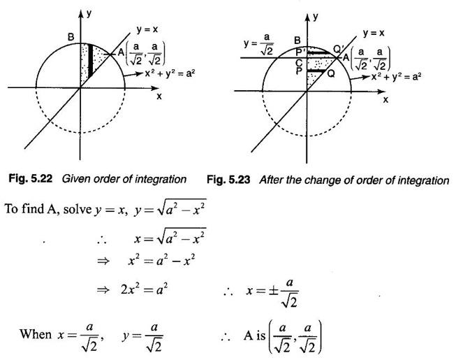
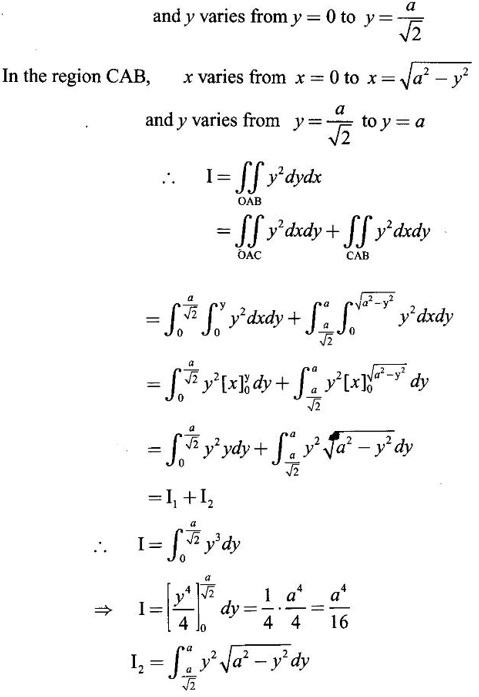
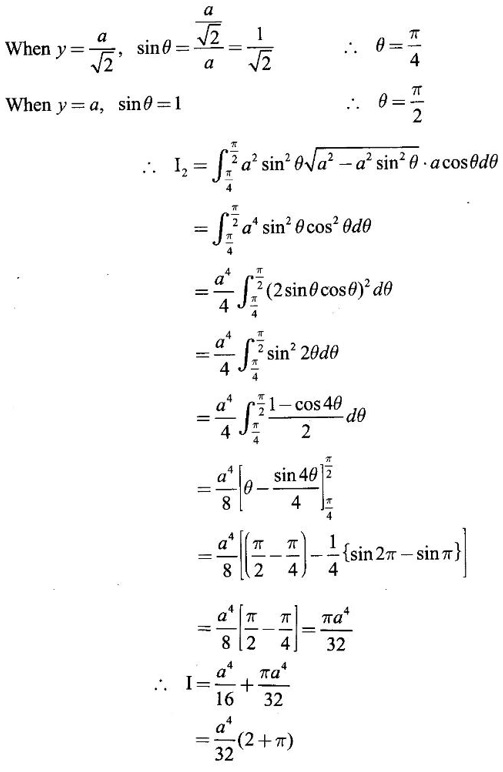
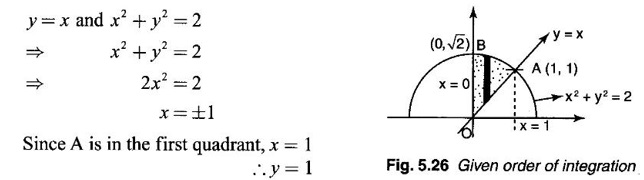
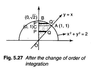
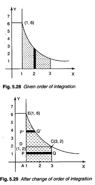
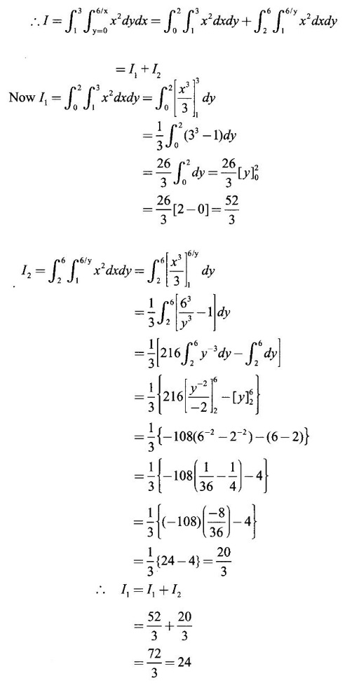
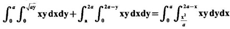
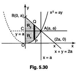
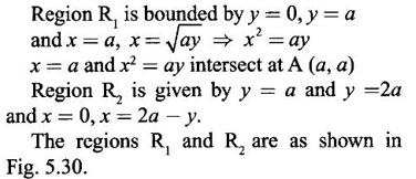
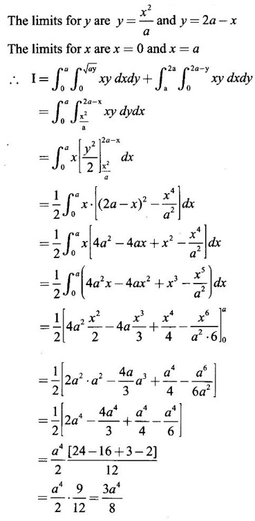
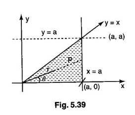
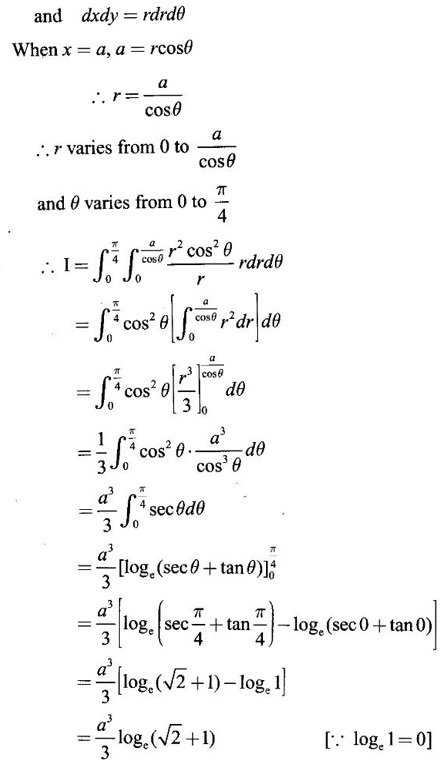
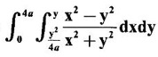
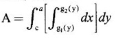
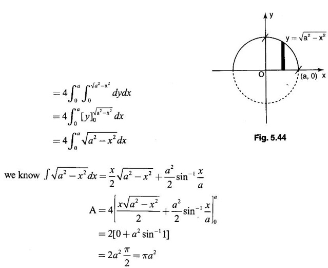
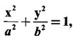
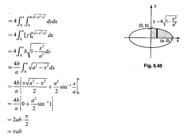
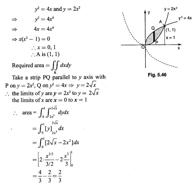
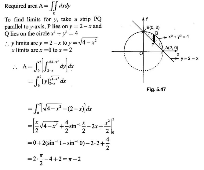
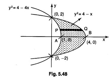
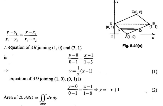
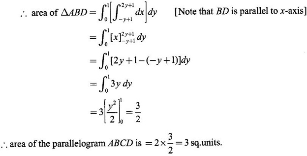
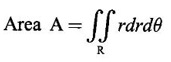
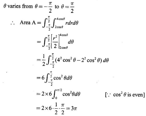
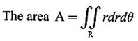
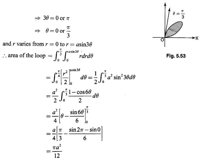
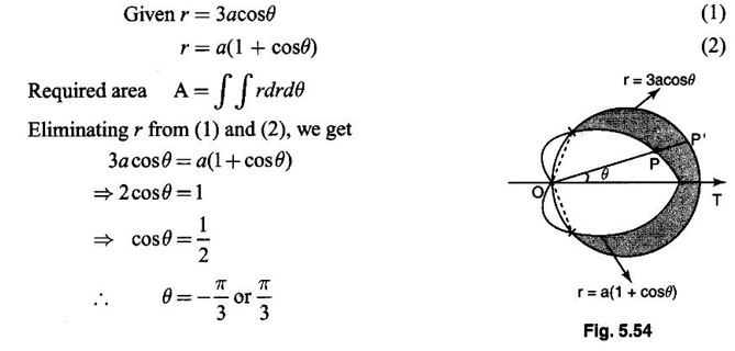
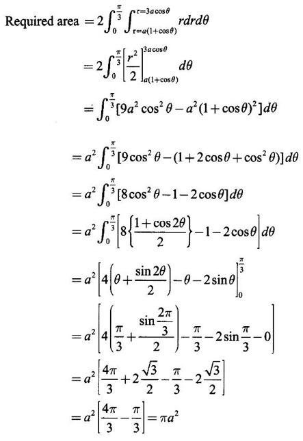
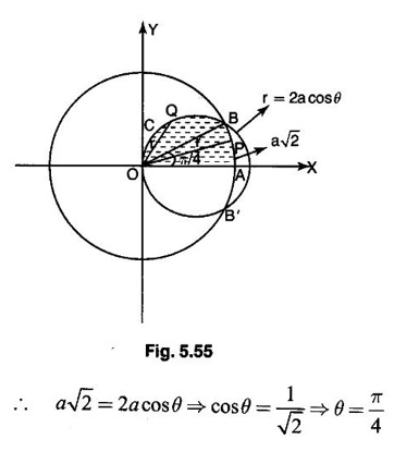
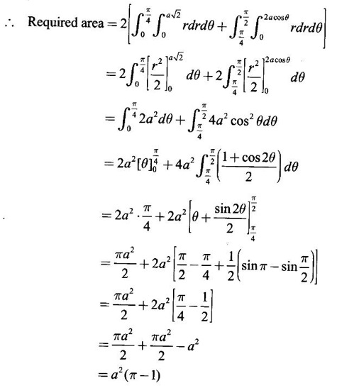
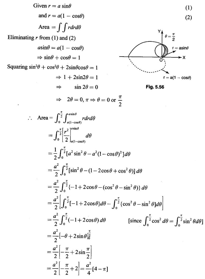
Unit - 5 Multiple Integrals DOUBLE INTEGRATION Double integrals occur in many practical problems in science and engineering. It is used in problems involving area, volume, mass, centre of mass. In probability theory it is used to evaluate probabilities of two dimensional continuous random variables. A double integral is defined as the limit of a sum. Let f(x, y) be a continuous function of two independent variables x and y defined in a simple closed region R. Sub-divide R into element areas ΔA1, ΔA2,...., ΔAn by drawing lines parallel to the coordinate axes. Let (x1, y1) be any point in ΔA1. Find the sum. Increase the number of sub-divisions indefinitely large i.e., n→∞ so that each ΔA1 → 0. In this limit, if the sum exists, i.e., Note The continuity of f(x, y) is a sufficient condition for the existence of double integral, but not necessary. The double integral exists even if finite number of discontinuous points are there in R, but it should be bounded. In practice, a double integral is computed by repeated single variable integration, integrate with respect to one variable treating the other variable as constant. Case 1: If the region R is a rectangle given by R= {(x, y)/a ≤ x ≤ b, c ≤ y ≤ d} where a, b, c, d are constants, then If the limits are constants the order of integration is immaterial, provided proper limits are taken and f(x, y) is bounded in R Case 2: If the region R is given by R = {(x, y) / a ≤ x ≤ b, g(x) ≤ y ≤ h(x)} where a and b are constants, then Here the limits of x are constants and the limits of y are functions of x, so we integrate first with respect to y and then with respect to x. Case 3: If the region R is given by R = {(x, y) / g(y) ≤ x ≤ h(y), c ≤ y ≤ d} where c and d are constants then Since the limits of x are functions of y, we integrate first w.r.to x and then w.r.to y Note (1) When variable limits are involved we have to integrate first w.r.to the variable having variable limits and then w.r.to the variable having constant limits. (2) When all the limits are constants, the order of dx, dy determine the limits of the variable. Example 1 Evaluate Solution Example 2 Show that Solution Example 3 Evaluate Solution Note We could write the integral in Example 3 as a product of two integrals because limits are constants and the functions could be factorised as x terms and y terms. This is not possible in Examples 1 and 2, even though the limits are constants. Example 4 Evaluate Solution Example 5 Evaluate Solution Example 6 Evaluate Solution Example 7 Evaluate Solution Given that the region R is bounded by the coordinate axes y = 0, x = 0 and the circle x2 + y2 = a2. So, the region of integration is the shaded region OAB as in Fig. 5.5. To find the limits for x, consider a strip PQ parallel to x-axis, x varies from x = 0 to x = When we move the strip to cover the region it moves from y = 0 to y = a. ⸫ limits for y are y = 0 to y = a. Example 8 Evaluate: Solution Given that the region of integration is bounded by y = x and y = x2 as in Fig. 5.6. To find the points of intersection solve y = x2 and y = x ⸫ x2 = x ⇒ x(x - 1) = 0 ⇒ x = 0 and x = 1 ⸫ y = 0,1 ⸫ Points are O (0, 0) and A (1, 1). We first integrate with respect to y. ⸫ take a strip parallel to y-axis, its lower end P is on y = x2 and upper end Q is on y = x. ⸫ limits for y are y = x2 and y = x. When we move the strip PQ to cover the region x varies from 0 to 1. Example 9 Evaluate Evaluate Solution Given that the shaded region OAB is the region of integration bounded by y = 0, x = 2a and the parabola x2 = 4ay as in Fig 5.7. We first integrate w.r.to y and then w.r.to x. To find the limits for y, we take a strip PQ parallel to the y-axis, its lower end P lies on y = 0 and upper end Q lies on ⸫ the limits for y are y = 0 to y = x2 / 4a. ⸫ When the strip is moved to cover the area, x varies from x = 0 to x = 2a. Example 10 Evaluate Solution Given that the region of integration is the triangle OAB as shown as Fig. 5.8. We first integrate w.r.to x and then w.r. to y. To find the limits for x, take a strip PQ parallel to x-axis. Its left end P is on x = y and right end Q is on x = 10y. ⸫ The limits for x are x = y and x = 10y. When the strip is moved to cover the region, y varies from 0 to 1. Example 11 Evaluate Solution The region R is the shaded region OAB. To find B, solve y2 = x and x + y = 2 Points are (+4, −2), (1, 1) But B is in first quadrant ⸫ B is (1, 1) and A is (2, 0) which is the point of intersection of y = 0 and x + y = 2. It is convenient to integrate first w.r.to x and hence we find the limits for x. ⸫ Take a strip PQ parallel to x-axis, P lies on y2 = x and Q lies on x + y = 2 ⇒ x = 2 - y ⸫ x limits are x = y2 and x = 2 - y When the strip is moved to cover the region, y varies from 0 to 1. Example 12 Evaluate Solution The parabola y = 4x - x2 = −(x2 - 4x) = −[(x − 2)2 - 4] ⇒ y – 4 = -(x - 2)2 ⇒ (x - 2)2 = -(y − 4) Its vertex is (2, 4), axis of symmetry is x = 2 and it passes through (0, 0) and downward. To find B, solve y = x and y = 4x - x2 ⇒ x = 4x - x2 ⇒ 3x - x2 = 0 ⇒ x2 - 3x = 0 ⇒ x(x - 3) = 0 ⸫ x = 0,3 When x = 3, y = 3 ⸫ B is (3, 3) ⸫ The region of integration is the shaded region OAB as in Fig. 5.10. We integrate first w.r.to y and then w.r.to x. To find y limits, take a strip PQ parallel to y-axis. P lies on y = x and Q lies on y = 4x - x2. ⸫ limits for y are y = x and y = 4x - x2. When the strip is moved to cover the region, x varies from 0 to 3. Example 13 Evaluate: Solution Given that the region of integration is the shaded region OAB as in Fig. 5.11. To find A solve x + y = 2 and y2 = x ⸫ A is (1, 1) and B is (0, 2) which is the point of intersection of x = 0 and x + y = 2. It is convenient to integrate with respect to y first and hence find y limits. Take a strip PQ parallel to y-axis. P lies on y2 = x and Q lies on x + y = 2. ⸫ the limits for y are y = √x and y = 2 - x. When the strip is moved to cover the region, x varies from 0 to 1. The double integral with variable limits for y and constant limits for x is For doing this we have to identify the region R of integration from the limits of the given double integral. Sometimes this region R may split into two regions R1 and R2 when we change the order of integration and hence the given double integral Example 1 Evaluate: Solution The region of integration is bounded by y = x, y = ∞o, x = 0, x = ∞. ⸫ The region is unbounded as in Fig. 5.12. In the given integral, integration is first with respect to y and then w.r.to x. After changing the order of integration, first integrate w.r.to x and then w.r.to y. To find the limits of x, take a strip PQ parallel to x-axis (see Fig. 5.13) with P on the line x = 0 and Q on the line x = y respectively. ⸫ the limits of x are x = 0 and x = y and Limits of y are y = 0 and y = ∞ Example 2 Evaluate by changing the order of integration Solution In the given integral, integration is first w.r.to y and then w.r.to x. After changing the order of integration, we have to integrate first w.r.to x and then w.r. to y. To find the points of intersection of the curves x2 = 4ay and y2 = 4ax, solve the two equations. x4 = 16a2 y2 = 16a2. 4ax = 64a3x Points of intersection are O(0, 0), and A is (4a, 4a) Now to find the x limits, take a strip PQ parallel to the x-axis (see Fig. 5.15) where P lies on y2 = 4ax and Q lies on x2 = 4ay. When the strip is moved to cover the region, y varies from 0 to 4a. Example 3 Change the order of integration in Solution ⇒ (x − a)2 + y2 = a2, which is a circle with (a, 0) as centre and radius a. The region of integration is the upper semi-circle OAB as in Fig. 5.17. The original order is first integration w.r.to x and then w.r.to y. After changing the order of integration, first integrate w.r.to y and then w.r.to x. To find the limits of y, take a strip PQ parallel to y-axis (see Fig. 5.17), where P lies on y = 0 and Q lies on the circle (x − a)2 + y2 = a2. Example 4 Evaluate Solution Example 5 Change the order of integration in Solution The region of integration is bounded by the lines x = 0, x = 1, y = x2, y = 2 - x. In the given integral, first integrate with respect to y and then w.r.to x. After changing the order we have to first integrate w.r.to x, then w.r.to y. To find A, solve y = x2, y = 2 - x ⇒ x2 = 2 - x ⇒ x2 + x – 2 = 0 ⇒ (x + 2)(x - 1) = 0 => x = -2, 1 Since the region of integration is OAB, x = 1 ⇒ y = 1 ⸫ A is (1, 1) B is (0, 2), which is the point of intersection of y-axis x = 0 and y = 2 -x Now to find the x limits, take a strip parallel to the x-axis. We see there are two types of strips PQ and P' Q' after the change of order of integration (see Fig. 5.21) with right end points Q and Q' are respectively on the parabola y = x2 and the line y = 2 - x. So, the region OAB splits into two regions OAC and CAB as in Fig. 5.21. Hence the given integral I is written as the sum of two integrals In the region OAC, x varies from 0 to √y y varies from 0 to 1 In the region CAB, x varies from 0 to 2 - y y varies from 1 to 2 Example 6 Evaluate: Solution x2 + y2 = a2, which is circle with centre (0, 0) and radius a. In the given integral, integration is first w.r.to y and then w.r.to x. After changing the order of integration, first integrate w.r.to x and then w.r.to y. After the change of order of integration to find x limits take a strip parallel to x-axis. We see there are two types of strips PQ and P'Q' (see Fig. 5.23) with Q on the line y = x and Q' on the circle x2 + y2 = a2 respectively. So, the region OAB splits into two regions OAC and CAB. Hence the integral I is written as sum of two integrals. In the region OAC, x varies from x = 0 to x = y Let y = a sin θ; ⸫ dy = a cos θ dθ Example 7 Change the order of integration in Solution The region of integration is OAB, bounded by the lines y = 0, y = 1 and x = y, x = 2 - y. To find A, solve x = y, x = 2 - y ⸫ x = 2 - x ⇒ 2x = 2 ⇒ x = 1 ⸫ y = 1 ⸫ Point A is (1, 1) In the given integral, integration is first with respect to x and then to w.r.to y. After changing the order of integration, first integrate w.r.to y and then w.r.to x. We see, there are two types of strips PQ and P'Q' (see Fig. 5.25) with ends Q and Q' lying on the lines y = x and x + y = 2 respectively. The region splits into two regions OAC and CAB (see Fig. 5.25). In the region OAC, y varies from y = 0 to y = x x varies from x = 0 to x = 1 In the region CAB, y varies from y = 0 to y = 2 - x x varies from x = 1 to x = 2 Example 8 Evaluate Solution The region of integration is bounded by lines x = 0, x = 1 and y = x, y = x2 + y2 = 2, which is a circle, with centre (0, 0) and radius √2. The region of integration is OAB as in Fig. 5.27. To find A, solve ⸫ A is (1, 1) and B is (0,√2), which is the point of intersection of x = x2 + y2 = 2 In the given integral, integration is w.r.to y first and then w.r.to x. After changing the order of integration, first integrate w.r.to x and then w.r.to y. To find x limits, take a strip parallel to x-axis. We see there are two strips PQ and P'Q' with ends Q, Q' on the line y = x and circle x2 + y2 = 2 respectively. So the region splits into 2 regions OAC and CAB. In the region OAC, x varies from 0 to y and y varies from 0 to 1 In the region CAB, x varies from 0 to Example 9 Change the order of integration and hence evaluate Solution The given region of integration is y = 0, y = 6/x and x = 1, x = 3. When x = 1, y = 6 When x = 3, y = 6/3 = 2 So the region of integration is the shaded region as in Fig. 5.29. The given order of integration is first with respect to y then w.r.to x. After changing the order of integration first integrate w.r.to x, then w.r.to y. To find x limits, take a strip parallel to the x-axis. We see there are two strips PQ and P'Q' with ends Q, Q' on the line x = 3 and on the rectangular hyperbola xy = 6 so, the region split into two regions ABCD and DCE. After change of order of integration, Example 10 Show that Solution The given integral I has some integrand defined over two region R1 and R2 given by the two double integrals. R1 is the shaded region OAC R2 is the shaded region CAB The line x + y = 2a also passes through A. Combining the two regions R, and R2 we get the shaded region OAB. In the given integral, we have to integrate first with respect to x and then w.r.to y. Changing the order integration, we first integrate w.r.to y, then w.r.to x. To find the y limits, take a strip PQ parallel to the y-axis. Change the order of integration in the following integrals and evaluate. To evaluate the double integral of f(r, θ) over a region R in polar coordinates, generally we integrate first w.r.to r and then w.r.to θ. So the double integral is However, whenever necessary, the order of integration may be changed with suitable changes in the limits. As in Cartesian, when we integrate w.r.to r, treat θ as constant. WORKED EXAMPLES Example 1 Evaluate Solution Important Formulae: Example 2 Evaluate Solution Example 3 Evaluate Solution We first integrate with respect to r. So take radius vector OPQ, then limits of r varies from P to Q. i.e., r varies from 2 sin θ to 4 sin θ. When PQ is varied to cover the area, θ varies from 0 to π Example 4 Evaluate Solution Example 5 Solution First integrate with respect to r Take a radial strip OP, its ends are r = 0 and Example 6 Evaluate Solution where the region A is the area between the circles r = 2 cos θ and r = 4 cos θ The area A is the shaded area in the Fig. 5.34 We first integrate w.r.to r. So take a radius vector OPQ r varies from P to Q ⸫ r varies from 2 cos θ to 4 cos θ When PQ is varied to cover the area A between r = 2 cos θ and r = 4 cos θ, θ varies from –π/2 to π/2 Example 7 Evaluate Solution Example 8 Evaluate Solution The evaluation of a double integral, sometimes become simpler if the variables of integration are transformed suitably into new variables. For example, from cartesian coordinates to polar coordinates or to some variables u and v. 1. Change of variables from x, y to the variables u and v. Let 2. Change of variable from Cartesian to polar coordinates Let Let x = r cos θ, y = r sin θ be the transformation from Cartesian to polar coordinates. WORKED EXAMPLES Example 1 Evaluate Solution Since x varies from 0 to ∞ and y varies from 0 to ∞, it is clear that the region of integration is the first quadrant as in Fig. 5.35 To change to polar coordinates put x = r cos θ, y = r sin θ ⸫ dxdy = rdrdθ and x2 + y2 = r2 cos2 θ + r2 sin2 θ = r2(cos2 θ + sin2 θ) = r2 ⸫ r varies from 0 to ∞ and θ varies from 0 to π/2 Example 2 Evaluate Solution which is a circle with centre (1, 0) and radius r = 1 and x varies from 0 to 2. ⸫ the region of integration is the upper semi-circle as in Fig. 5.36 To change to polar coordinates, put x = r cos θ, y = r sin θ Example 3 By changing into polar coordinates, evaluate the integral Solution ⇒ x2 + y2 - 2ax = 0 ⇒ (x − a)2 + y2 = a2 which is a circle with centre (a, 0) and radius r = a x varies from 0 to 2a ⸫ the region of integration is the upper semi circle as in Fig. 5.37. To change to polar coordinates put x = r cos θ, y = r sin θ. ⸫ dxdy = rdrdθ Example 4 Evaluate Solution The region of integration is as in Fig. 5.38. To change to polar coordinates, put x = rcos θ, y = r sin θ ⸫ dxdy = rdrdθ x2 + y2 = r2 ⸫ x2 + y2 = ax ⇒ r2 = ar cos θ ⇒ r(r – a cos θ) = 0 ⸫ r = 0 and r = a cos θ ⸫ r varies from 0 to a cos θ and θ varies from 0 to π/2 Example 5 Evaluate Solution Given, Limits for x are x = y and x = a Limits for y are y = 0, y = a ⸫ The region of integration is as in Fig. 5.39. To change to polar coordinates, put x = rcos θ, y = r sin θ ⸫ x2 + y2 = r2 Example 6 Evaluate Solution Now y2 = 4ay ⇒ (y - 4a) = 0 ⇒ y = 0, y = 4a ⸫ x = 0, x = 4a ⸫ Points are (0, 0), (4a, 4a) ⸫ the region of integration is the shaded region as in Fig. 5.40 which is bounded by y2 = 4ax and y = x. To change to polar coordinates, put x = rcosθ, y = rsinθ ⸫ dxdy = rdrdθ x2 + y2 = r2 x2 - y2 = r2cos2θ - r2sin2θ = r2 (cos2θ - sin2θ) = r2cos2θ y2 = 4ax becomes r2sin2θ = 4a · rcosθ ⇒ r(r sin2θ - 4a cosθ) = 0 ⇒ r = 0 and r sin2θ - 4a cosθ = 0 Example 7 Evaluate Solution which is circle with centre (0, 0) and radius a Limits for y are y = 0 and y = a ⸫ the region of integration is as in Fig. 5.41 bounded by y = 0, y = a and x2 + y2 = r2 ⸫ x2 + y2 = a2 ⇒ r2 = a2 ⇒ r = ± a ⸫ In the given region, r varies from 0 to a and θ varies from 0 to π/2 Example 8 Evaluate Solution The region of integration is the positive quadrant of x2 + y2 = 4, as in Fig. 5.42 x2 + y2 = 4 is a circle with centre (0, 0) and radius = 2 ⸫ In the given region, r varies form 0 to 2 and θ varies from 0 to π/2. Example 9 Evaluate Solution Now x2 + y2 = 2ax ⇒ r2 = 2arcos θ ⇒ r2 - 2 arcos θ = 0 ⇒ r(r - 2a cos θ) = 0 ⸫ r = 0, r = 2a cos θ ⸫ r varies from 0 to 2a and θ varies from 0 to π/2 Example 10 Transforming to polar coordinates evaluate the integral Solution Polar Coordinates 6. Area as double integral (a) Area as double integral in cartesian coordinates Double integrals are used to compute area of bounded plane regions. The area A of a plane bounded region R in cartesian coordinates is (i) If the region R is bounded by curves y = f1(x), y = f2(x) and lines x = a, x = b where a and b are constants, (ii) If the region R is bounded by curves x = g1(y), x = g2(y) and line y = c, y = d where c and are constants, then WORKED EXAMPLES Example 1 Find the area of a circle of radius a by double integration. Solution The equation of a circle of radius a is x2 + y2 = a2 The area in the four quadrants are equal, because of the symmetry of the curve w.r.to both axes. ⸫ Area A = 4 × area in the I quadrant Example 2 Find the area bounded by the ellipse Solution Equation of the ellipse is By the symmetry of the curve, the area of the ellipse is A = 4 × Area in the first quadrant Example 3 Using double integral find the area enclosed by the curves y = 2x2 and y2 = 4x. Solution The region of integration is the shaded region (as in Fig. 5.46) bounded by y2 = 4x and y = 2x2 To find A, solve the equations Example 4 Find the smaller of the areas bounded by y = 2 - x and x2 + y2 = 4 using double integral. Solution The region R is the shaded part in Fig. 5.47. Example 5 Find the area bounded by the parabola y2 = 4 x and y2 = 4 - 4x as a double integral and evaluate it. Solution y2 = -(x - 4) is a parabola with vertex (4, 0) and towards -ve x-axis, axis of symmetry x-axis. y2 - 4(x - 1) is a parabola with vertex (1, 0) and towards -ve x-axis, axis of symmetry x-axis. To find their points of intersections solve 4 - x = 4 - 4x ⇒ x = 0 ⸫ y2 = 4 ⇒ y = ±2 ⸫ Points are (0, 2), (0, −2) Draw the graph and determine the region. The region is the shaded region as in Fig. 5.48. Both curves are symmetric about x-axis. ⸫ Required area A = 2 Area above the x-axis It is convenient to take strip PQ parallel to the x-axis. P lies on y2 = 4 - 4x and Q lies on y2 = 4 - x Example 6 Find the area between the parabola y = 4x - x2 and the line y = x by double integration. Solution Points of intersection are O(0, 0), A(3, 3) The region is bounded by the line y = x and parabola y = 4x - x2 is the shaded region as in Fig. 5.49. It is convenient to take strip PQ parallel to y axis. P lies on y = x and Q lies on y = 4x - x2 The limit of y are y = x to y = 4x - x2 The limits of x are x = 0 to x = 3 Example 7 Using double integration find the area of the parallelogram whose vertices are A(1, 0), B(3, 1), C(2, 2), D(0,1) Solution: Area of the parallelogram ABCD = 2 (area of the triangle ABD) We shall find the equations of AB and AD. We know equation of line joining the points (x1, y1) and (x2, y2) is Take a strip PQ parallel to x-axis with P on (2). ⸫ x = -y + 1 and Q is (1) ⇒ x = 2y + 1 1. Find the area bounded by the parabola x2 = 4y and the straight line x - 2y + 4 = 0. 2. Evaluate the area bounded by y = x and y = x2. 3. Evaluate the area bounded by y2 = 4ax and x2 = 4ay. 4. Evaluate the area bounded by y = 4x − x2 and y = x. 5. Evaluate the smaller area bounded by 6. Evaluate the smaller area bounded by x2 + y2 = 4 and x + y = 2. 7. Evaluate the area bounded by y2 = 4x, x + y = 3 and the X-axis. 8. Evaluate the area bound by y = 9. Find the area common to y2 = x and x2 + y2 = 4. 10. Find the area bounded by y2 = 4 - x, y2 = x. 11. Find the area of the curve a2y2 = x2(2a - x). (b) Area as double integral in polar coordinates As double integral, area in polar coordinates is where R is the region for which area is required. WORKED EXAMPLES Example 1 Find the area bounded between r = 2cos θ and r = 4cos θ. Solution where the region R is the area between the circles r = 2cosθ and r = 4cosθ The area is the shaded region as in Fig. 5.50. We first integrate w.r.to r and so we take the radius vector OPQ. When PQ is moved to cover the area A, r varies from r = 2cosθ to r = 4cosθ, and Example 2 Find the area of the cardioid r = a(1 a(1 - cosθ). Solution Given r = a(1 – cos θ) where region R is the area of the cardioid. First we integrate w.r.to r, Take a radial strip OP, its ends are at r = 0 and r = a(1 – cos θ) When it is moved to cover the area, θ varies from 0 to π. Since the curve is symmetric about OX. Example 3 Find the area of one loop of the leminiscate r2 = a2cos2θ. Solution Given r2 = a2cos2θ R is the region as in Fig. 5.52. Since the loop is symmetric about the initial line, required area is twice the area above the initial line. First we integrate w.r.to r In this region, take a radial strip OP, its ends are r = 0 and r = Example 4 Find the area of a loop of the curve r = asin3θ. Solution Given r = asin3θ But the loop is formed by two consecutive values of θ when r = 0 when r = 0, a sin3θ = 0 Example 5 Find the area which is inside the circle r = 3acosθ and outside the cardioid r = a(1 + cos θ). Solution Required area is shaded region as in Fig. 5.54. Since both the curves are symmetrical about the initial line, required area is twice the area above the initial line. In this region take a strip PP'. When it moves, it will cover the required area. ⸫ r varies from a(1 + cos θ) to 3acos θ and θ varies from 0 to π/3. Example 6 Find the area common to r = a√2 and r = 2acos θ. Solution Given r = a√2 (1) and r = 2acosθ (2) (1) is circle with centre (0, 0) and radius a√2 (2) is a circle with centre (a, 0) and radius a Solve (1) and (2) to find the point of intersection. Since the circles are symmetrical about the initial line OX, required area = 2 area OABC = 2 [Area OAB + area OBC] In OAB, take a strip OP. When OP moves it covers the area OAB. ⸫ r varies from 0 to a√2 and θ varies from 0 to π/4. In the area OBC, take a strip OQ. When OQ moves it covers the area OBC Example 7 Find the area inside the circle r = asin θ but lying outside the cardiod r = a(1 - cos θ). Solution EXERCISE 1. Find the area bounded between r = 2sin θ and r = 4sin θ. 2. Find the area of one loop of r = acos3 θ. 3. Find the area that lies inside the cardioid r = a(1 + cos θ) and outside the circle r = a. 4. Find the area of the cardioid (i) r = a(1 + cos θ), (ii) r = 4(1 + cos θ) 5. Find by double integration, the area lying inside the cardioid r = 1 + cos θ and out the parabola r(1 + cos θ) = 1. 6. Calculate the area included between the curve r = a(sec θ + cos θ) and its asymptote. ANSWERS TO EXERCISE 1. Double integrals in cartesian coordinates

 exists, it is called the double integral of f(x, y) over the region R and it is denoted by
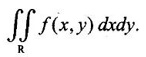
2. Evaluation of double integrals

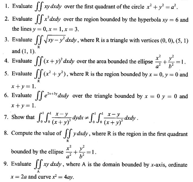
WORKED EXAMPLES
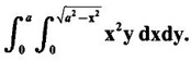
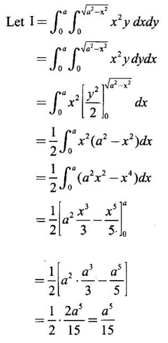
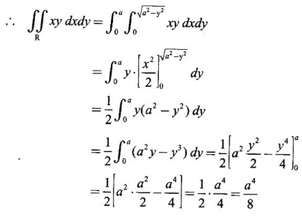
 over the positive quadrant of the circle x2 + y2 = a2.
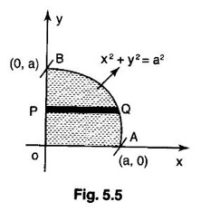

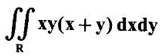 over the area between y = x2 and y = x.
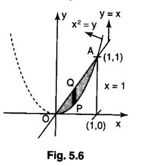

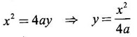
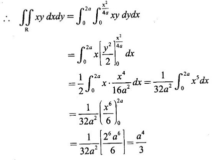
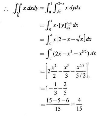
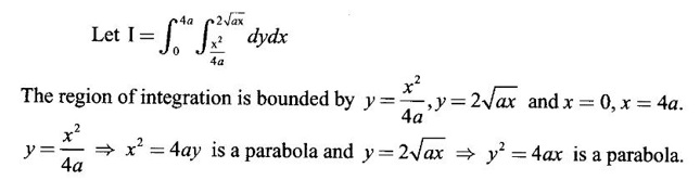
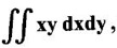 where A is the region bounded by x = 2a and the curve x2 4ay.
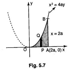
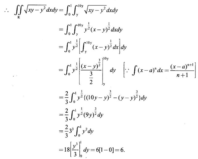
 where R is the triangle with vertex (0, 0), (10, 1), (1, 1).
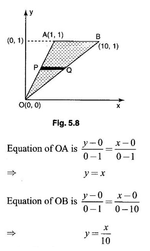
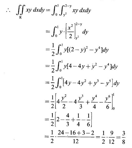
 where R is the region bounded by the parabola y2 = x, the x-axis and the line x + y = 2, lying on the first quadrant.
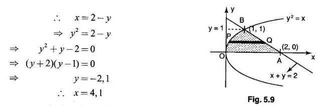
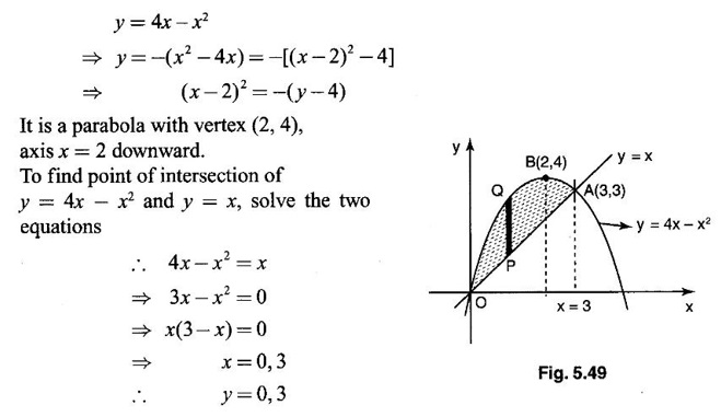
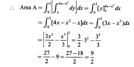
 over the region R bounded by y = x and y = 4x - x2.
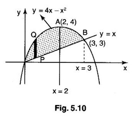

 over the region R bounded by y2 = x and the lines x + y = 2, x = 0, x = 1.
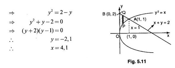
EXERCISE
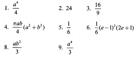
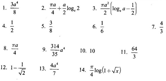
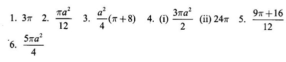
ANSWERS TO EXERCISE
3. Change of order of integration
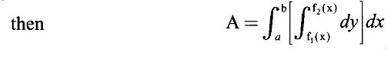
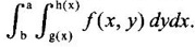 To evaluate this integral, we integrate first w.r.to y and then w.r.to x. This may sometimes be difficult to evaluate. But change in the order of integration will change the limits of y from c to d where c and d are constants and the limits of x from g1 (y) to h1 (y). The double integral becomes
 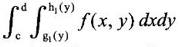 and hence the evaluation may be easy. To evaluate this integral, we integrate first w.r.to x and then w.r.to y. This process of changing a given double integral into an equal double integral with order of integration changed is called Change of order of integration.
 will be the sum of two double integrals.
WORKED EXAMPLES
 by changing the order of integration.
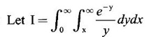

 and then evaluate it.
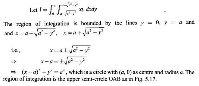

 by changing the order of integration.
 and hence evaluate.

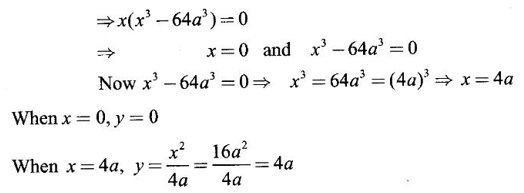
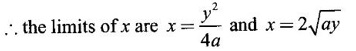
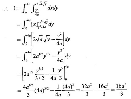
 by changing the order of integration.
 and hence evaluate.

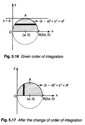
 by changing the order of integration.

 and y varies from 1 to √2
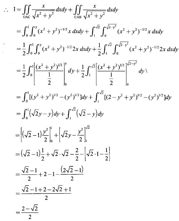
 and hence evaluate.
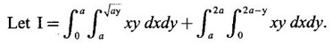
EXERCISE
ANSWERS TO EXERCISE
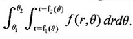
4. Double integral in polar coordinates
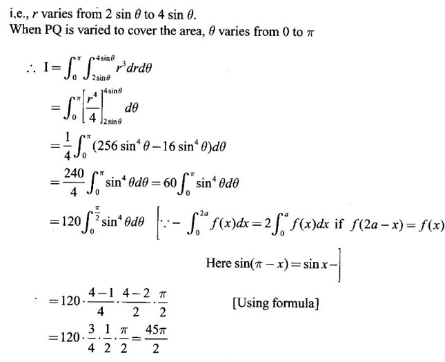
 where A is the area between the circles r = 2 sin θ and r = 4 sin θ.
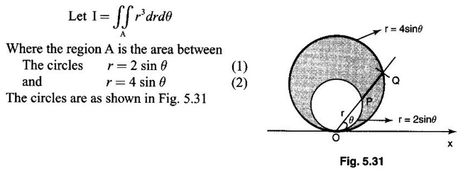
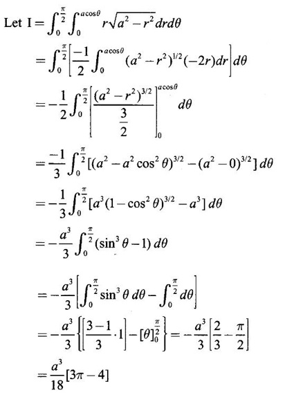
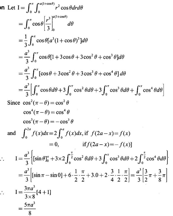
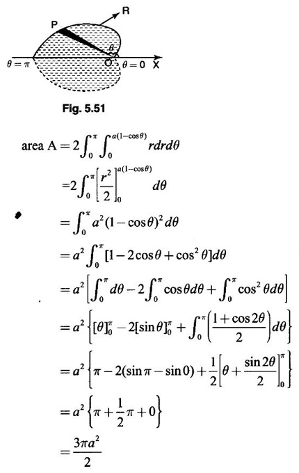
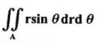 over the area of the cardioid r = a(1 + cos θ) above the initial line.

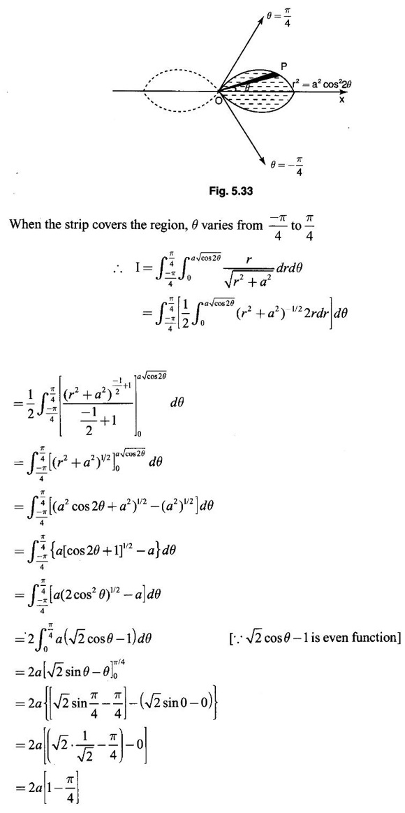
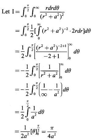
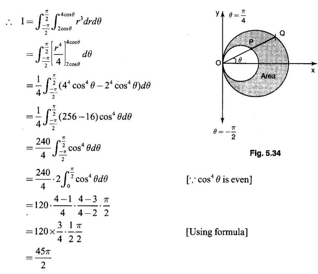
 over the area bounded between the circles r = 2 cos θ and r = 4 cos θ.
5. Change of variables in double integral
 be the given double integral.
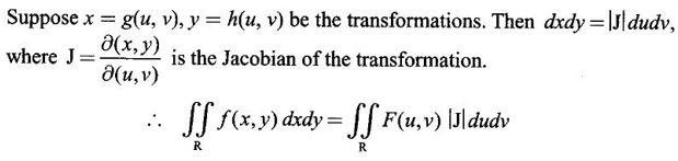
 be the double integral.
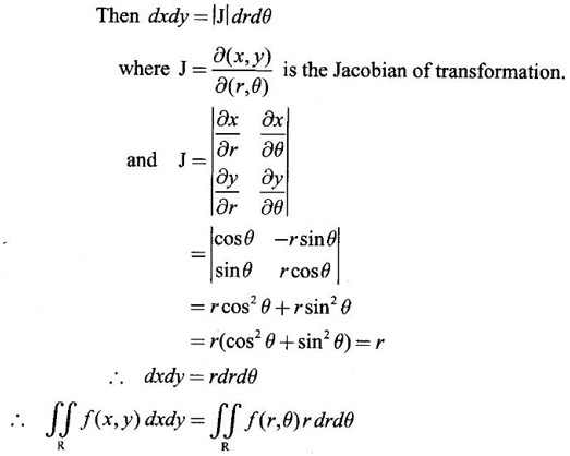
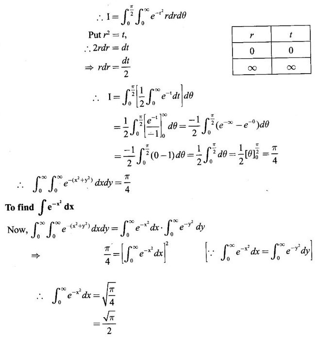
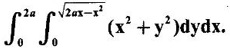
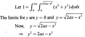
 by changing to polar coordinates and hence evaluate
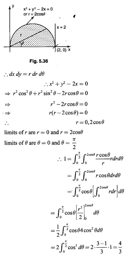
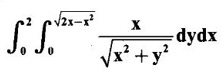 by changing into polar coordinates.
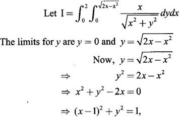
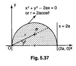
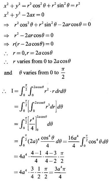
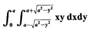
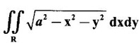 where R is the semi-circle x2 + y3 = ax in the I quadrant, changing to polar coordinates.
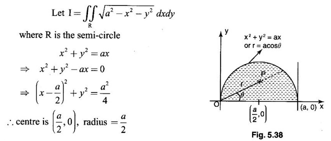

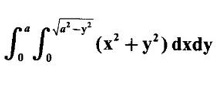
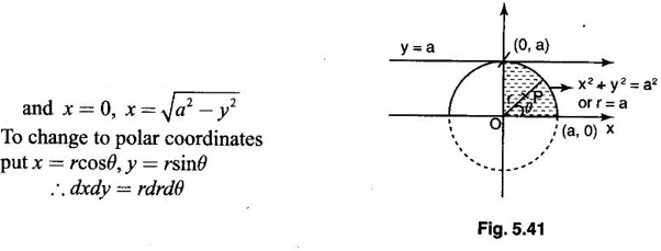
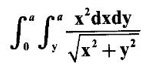 by changing to polar coordinates.
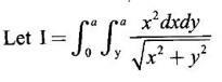
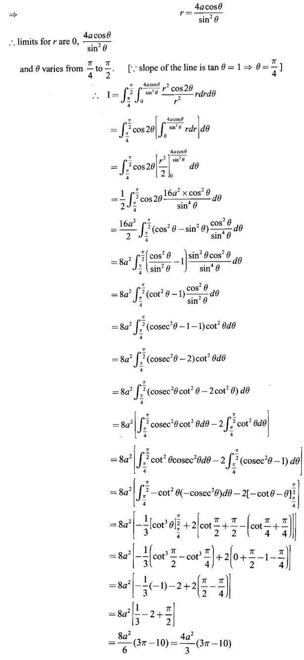
 by changing to polar coordinates.
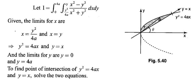
 by changing into polar coordinates.
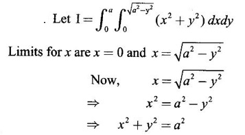
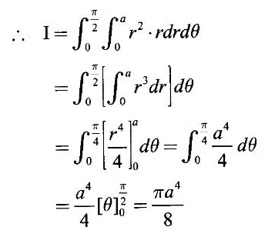
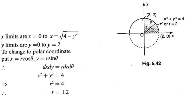
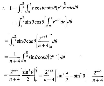
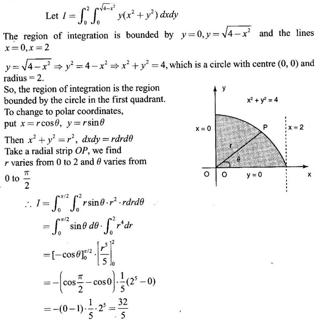
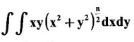 over the positive quadrant of x2 + y2 = 4, supposing n + 3 > 0.
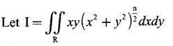
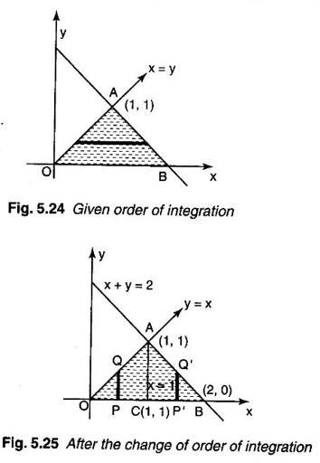
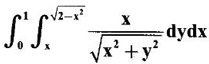
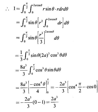
 where R is the region bounded by the semi-circle x2 + y2 = 2ax and the x-axis and the lines y = 0 and y = a.
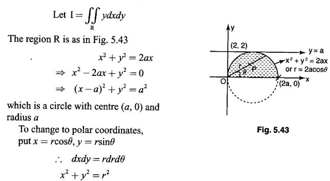
EXERCISE

ANSWERS TO EXERCISE
 using double integration.
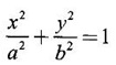

EXERCISE
ANSWERS TO EXERCISE


Matrices and Calculus: Unit V: Multiple Integrals : Tag: : Worked Examples, Exercise with Answers - Double Integration
Related Topics
Related Subjects
Matrices and Calculus
MA3151 1st semester | 2021 Regulation | 1st Semester Common to all Dept 2021 Regulation