Strength of Materials: Unit IV: Deflection of Beams
Deflection of Beams
introduction
The cross-section of a beam must be strong enough to resist the bending and shear stresses which are produced by various loads. This criterion is called strength criterion.
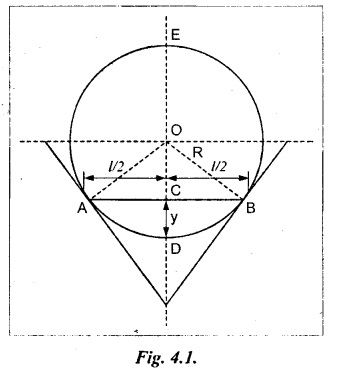
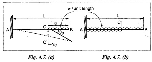
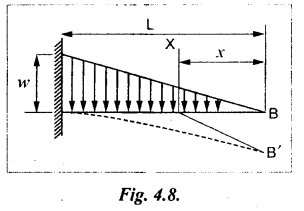
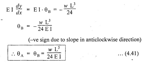
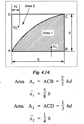
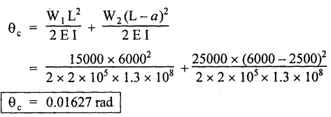
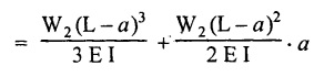
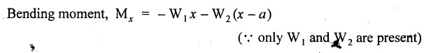
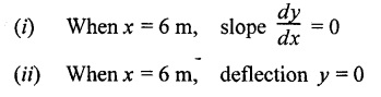
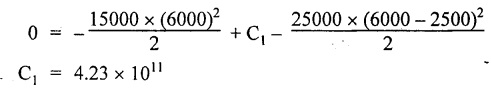
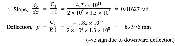
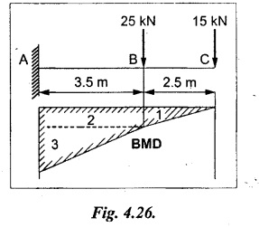
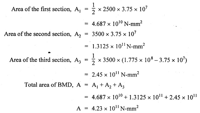
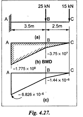
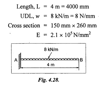
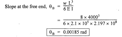
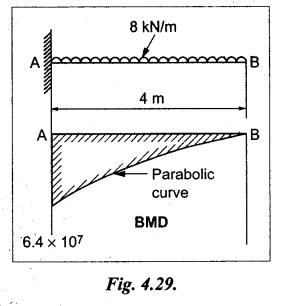
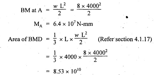
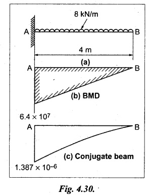
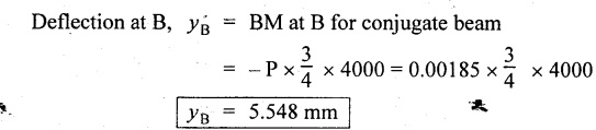
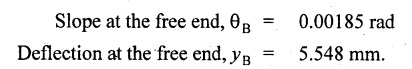
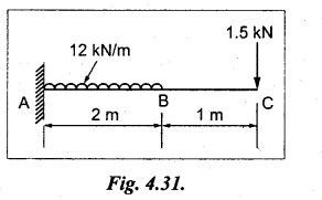
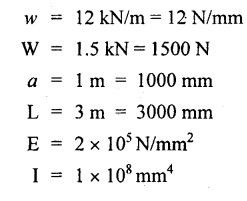
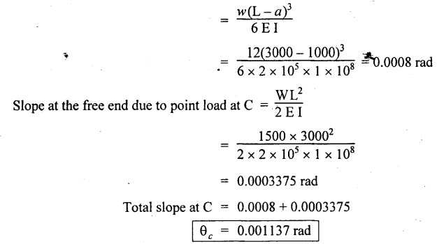
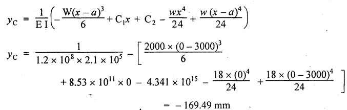
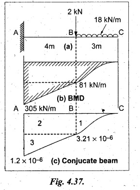
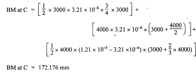
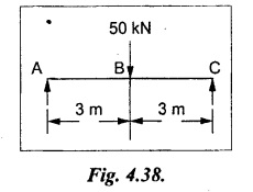
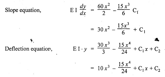
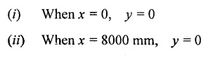
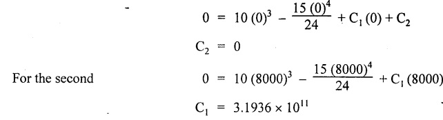
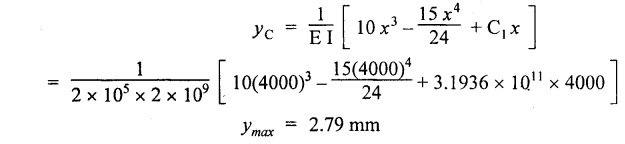
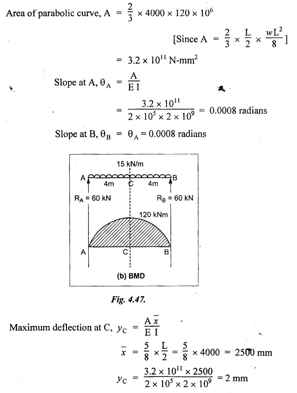
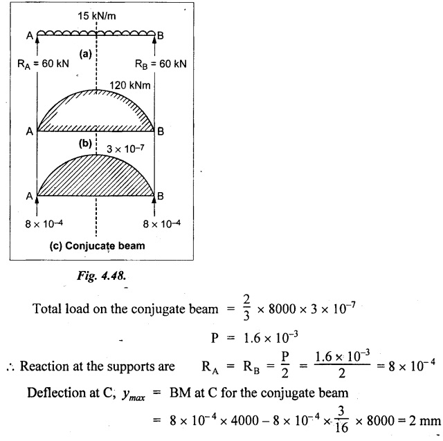
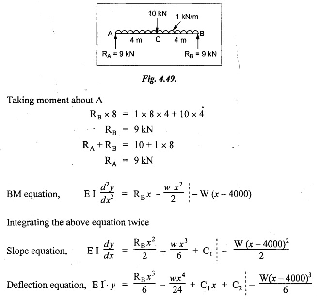
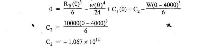
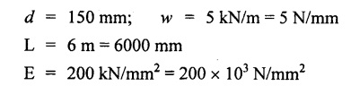
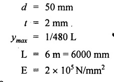
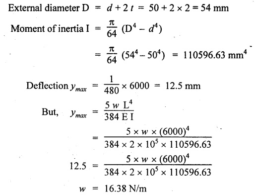
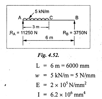
Chapter 4 DEFLECTION OF BEAMS • Double Integration Method • Macaulay's Method • Moment Area Method • Conjugate Beam Method • Strain Energy Method • Maxwell's Reciprocal Theorem • Strain Energy • Solved Problems • Two Marks Q & A DEFLECTION OF BEAMS The cross-section of a beam must be strong enough to resist the bending and shear stresses which are produced by various loads. This criterion is called strength criterion. Another criterion which is equally important is called deflection of the beam. The maximum deflection of the beam must not exceed a given limit i.e., the beam must be stiff enough to resist against deflection. Thus, the stiffness, of the beam which is inversely proportional to the deflection is the second criterion of beam design. "Stiffness” of a beam is a measure of the resistance offered by the beam to deflection from its original position. The ratio of span to the deflection of the beam is known as the "Stiffness factor". The allowable ratio of deflection to span varies between 1/2000 to 1/360. Deflection is caused mainly due to bending moment and to a small measure due to shear force. In most of the cases it becomes necessary to design a machine member or a structure to minimize deflection. Thus it becomes necessary to determine the deflection of the member. Deflection of beams may be determined analytically by the following methods. (i) Double integration method (ii) Macaulay's method (iii) Moment area theorem method (iv) Conjugate beam method In actual cases of loading, the beam does not bend to a true arc of a circle but depending upon the load nature it bends in the form of flat curve. But we can safely assume that the axis of the beam bends to a circle of radius R where the bending moment is M. Consider a beam ACB of length l, bent in the form of a circular arc ADB. Let CD is the deflection of beam at its mid span which is equal to y and OB be the radius of curvature equal to R as shown in Fig.4.1. From geometry of the circle, Consider a small portion of the beam PQ equal to ds along the curve as shown in Fig.4.2. From the geometry of the Fig.4.2, If x and y be the coordinates of point P, then Since Ψ is very small, then tan y = y Differentiating the above equation with respect to x, From bending equation, Differentiating the above equation with respect to x, we get Again differentiating the above equation with respect to x, we get, Uniform load, Hence the relation between curvature, slope, deflection etc., at a section is given Deflection = y The bending moment at any point is given by the differential equation (4.3). Integrating the above equation, we get This is the slope equation. Integrating the above equation twice, we get This is the deflection equation. Therefore, if we integrate the bending moment equation we get the slope at any point. On further integration we get the value of deflection at any point. Thus it is called Double-integration method. A cantilever AB of length L fixed at one end A and free at end B and carrying a point load W at free end B as shown in Fig.4.3. Consider a section Xát a distance x from the free end. BM at that section. We know that, Equating the above two equations Integrating the above equation Integrating again, we get Where C1, and C2 are constant of Integrations. Their values obtained from the following boundary conditions, Applying the fist BC: to the equation (i) Applying the second B.C. to the equation (ii) Substituting the C1 value in equation (i) we get the slope equation at a point Maximum slope can be determined by substituting x = 0 in the above equation Substituting the values of C1 and C2 in equation (ii), we get the deflection equation at any point. The maximum deflection occurs at free end. Therefore, maximum deflection Ув can be determined by substituting x = 0 in the above equation. A cantilever AB of length L fixed at A and free at B, carrying a point load W at a distance of 'a' from the free end B as shown in Fig.4.4. The portion AC will bend into AC' while the portion CB remains straight but displaced to C'B'. Therefore the portion AC of the cantilever may be taken as similar to a cantilever of previous case (i.e., Art 4.1.5 load at free end). From equation (4.5), Since the portion CB of the cantilever is straight, therefore, From the geometry of the Fig.4.4, we find When load is acting at mid span of the cantilever A cantilever AB of length L fixed at end A and free at B carrying a UDL of w per unit length over the whole, is shown in Fig.4.5. Consider a section X at a distance x from the free end B. The C1 and C2 values are obtained from the following boundary conditions. Applying first boundary condition (B.C) to the equation (i), Substituting the C1 value in equation (i), we get the slope equation at any point Maximum slope can be determined by substituting x = 0 in equation (4.13). Substituting C1 and C2 values in equation (ii), we get the deflection equation at any point Maximum deflection occurs at the free end. Therefore maximum deflection can be determined by substituting x = 0 in equation (4.15). A cantilever AB of length L fixed at A and free at B and carrying a UDL of w unit length for a distance of (L − a) from the fixed end, is shown in Fig.4.6. The portion AC will bend into AC', while the portion CB will remains straight, but will displace to C'B'. Therefore the portion AC of the cantilever may be taken as similar to previous case (i.e., Art 4.1.7 UDL throughout the span). From geometry of the fig, we have Deflection at B when UDL acting half of the length A cantilever AB of length L fixed at A and free at B and carrying a UDL of w/m length for a distance of 'a' from free end, is shown in Fig.4.7(a). The slope and deflection at the end B is determined as follows, (i) Consider the whole cantilever AB loaded with UDL of w per m as shown in Fig.4.7 (b). (ii) Then superimpose on upward UDL of w per unit length from A to C as shown in Fig.4.7(b). (iii) Now, slope at B = slope due to downward UDL over entire length - slope due to upward UDL from A to C. Deflection at B = Deflection due to UDL of entire length - Deflection due to upward UDL from A to C. From equation (4.14), From equation (4.18), Similarly, From equation (4.16), Downward deflection due to UDL of entire length From equation (4.20), Upward deflection of point B due to UDL of length AC A cantilever of length L fixed at A and free at B and carrying UVL from O at B to w per unit length at the fixed end A, is shown in Fig.4.8. Consider a section X, at a distance of x from the free end B. Substituting the C1 value in equation (i) we get the slope equation at any point The maximum slope occurs at the free end. Therefore, for maximum slope, substitute x = 0 in equation (4.24) Applying the second B.C. to the equation (ii) Substituting the values of C1 and C2 in equation (ii) The maximum deflection occurs at the free end. Therefore, the maximum deflection Ув can be determined by substituting x = 0 in the equation (4.26). A simply supported beam AB of length L and carrying a point load W at its mid span is shown in Fig.4.9. Equating the above two equations The value of C1 and C2 can be found by applying the following conditions, Applying the first B.C. to the equation (i) Substituting C1 value in equation (i) we can get the slope equation at any point Slope is maximum at A or B. Therefore, the maximum slope is obtained by substituting, x = 0 in the above equation Applying the second B.C to the equation (ii) 0 = 0 + 0 = C2 Substituting the values of C1 and C2 in equation (ii), we can get the deflection at any point, Deflection is maximum at the centre of the beam (i.e., at C). Therefore by substituting x = L/2, we can get the maximum deflection. A simply supported beam, AB of length L and carrying a point load W at a distance 'a' from support A and at a distance b from support B are shown in Fig.4.10(a). (a) Now, consider a section X at a distance x from B in length CB. The bending moment at this section is given by The C1 and C2 values are obtained by applying boundary conditions, The above equations are useful only when (b) Now, consider a section X at a distance x from B in length AC. The bending moment at section X, The C3 and C4 values are obtained by applying the following boundary conditions, Substituting the first B.C. in the equation (v) Applying the second B.C in equation (vi) Substituting C3 and C4 values in equations (v) and (vi) The above equations are useful when θC is known. To find out the value of θC, equate the deflection equations obtained from AC and CB (i.e., equation (iv) and (vii)) by substituting x = b. Because when we substitute x = b in both the equations, these will give the deflection value at B. Substituting the value of EI θC in equation (iii) Slope equation in section BC Similarly slope equation in section AC is Slope is maximum at B. Thus for maximum slope, substituting x = 0 in the above equation Deflection at any point in CB, substitute the value of E I θC in equation (iv). Deflection at any point in section CB Similarly Deflection at any point in section AC, For deflection at C, substitute x = b in the above equation Deflection at the point of application of load Maximum deflection Since 'b' is more than 'a' maximum deflection will be in section CB. When the deflection is maximum, slope For maximum deflection, substitute the value of x in equation (4.35) If 'a' is more than 'b', then the above equation becomes A simply supported beam of length L and carrying a UDL of w per m length over the entire length is shown in Fig.4.11. Consider a section X at a distance x from B. The bending moment at this section is given by Equating above equation with equation (4.3) Integrating the above equation, The value of C1 and C2 can be determined by applying the following boundary conditions, Applying the first B.C. to the equation (i) By substituting C1 in equation (i) we get the slope equation at any point The maximum slope occurs at A and B. Thus for maximum slope substituting x = 0 in the above equation Applying the second B.C. to the equation (ii) 0 = C2 ⸫ C2 = 0 By substituting the values of C1 and C2 in equation (ii), we can get the deflection equation at any point, The deflection is maximum at mid-point C. Therefore maximum deflection is obtained by substituting x = L/2 in the equation (4.42). In the previous double integration method for finding the slope and deflection for simply supported beam loaded with many point loads and UDL is very tedious and laborious. Mr. W.H. Macaulay derived a method of continuous expression for bending moment and integrating in such a way, that the constants of integration are valid for all sections of the beam; even though the law of bending moment varies from section to section. Consider a beam simply supported and loaded as shown in Fig.4.12. For any section between A and C at a distance x from A, Bending moment, M = RA x. This equation holds good for all values of x between x = 0 and x = a. For any section between C and D at a distance x from A. Bending moment, This equation holds good for all values of x between x = a and x = b. For any section between D and E at a distance x from A, Bending moment, This equation holds good for all values of x between x = b and x = c. For any section between E and F and at a distance x from A. Bending moment, For any section between F and B at a distance x from A. Bending moment, If we use the double integration method, each of the 5 equations integrated twice and we get total of 10 constants which are to be determined. This can be found from boundary conditions. However, in this way the solution of the problem.would become too lengthy and tedious. This difficulty can be eliminated by using a mathematical technique called Step function. The step function is of the form In this method at any section of the beam, the bending moment is given by NOTE: (a) While using this method, the section x is to be taken in the right side last part of the beam. (b) The UDL has to continue always upto the right end of the beam. If it is not so as in our case, a negative load (upward) may be applied in the portion of the beam (refer Fig.4.12(b)) left uncovered by the given UDL. This will balance the extended UDL. The above equation written in such a manner that the magnitude of x goes on increasing when the law of loading changes, and additional expressions appear. For values of x between x = 0 and x = a, only the first term of the above equation should be considered. For values of x between x = a and x = b, only the first two terms of the above equation should be considered and so on. Integrating equation (4.44), we get the general expression for slope. It is very important to note the following point when integrating (a) The constant of integration C1 should be written after the first term of the above equation. (b) The quantity (x − a) should be integrated as (c) The constant C1 is valid for all values of x. Integrating equation (4.45), we get the deflection equation Same procedure as in previous case is followed when integrating the above equation. The constants C1 and C2 can be evaluated if the boundary conditions are known. The application of Macauley's method is shown in problems. Consider a beam AB carrying some type of loading, and hence subjected to bending moment as shown in Fig.4.13. Let the beam bend into A P1, Q1 B and due to the load acting on the beam A be a point of zero slope and zero deflection. Consider an element PQ of small length dx at a distance of x from B. The corresponding points on the deflected beam are P1 Q1. Let, R - Radius of curvature of deflected beam dθ - Angle included between the tangent P1 and Q1 M - Bending moment between P and Q dx - Length of PQ θ - The angle in radians, included between the tangents drawn at the extremities of the beam i.e., at A and B facing the reference line. From geometry of the bend up beam Section P1 Q1, we have From bending moment equation Substituting R value in dθ equation, Since A is point of zero slope, the total slope at B is obtained by integrating the above equation between the limits O and L. We know that M . dx represents the B.M diagram of length dx. Hence, In case, slope at A is not zero, then "Total change of slope between B and A equals the area of B.M diagram between B and A divided by the flexural rigidity EI". Deflection due to the bending of the portion PQ. Substituting the value of de from above equation (i) Since the deflection at A is assumed to be zero, the total defection at B is obtained by integrating the above equation between the limits 0 and L. But x × M × dx represents the moment of area of the BM diagram of length dx about point B. This is equal to the total area of BM diagram multiplied by the distance of the C.G of the BM diagram area from B. In case the point A is not a point of zero slope and deflection. "The deflection of B with respect to the tangent at A equal to B, the first moment about B of the area of the B.M diagram between B and A". The results given in the equations (4.47) for slope and (4.48) for deflection are known as Mohr's theorems. These are stated as Theorem 1: The change of slope between any two points is equal to the net area of the B.M diagram between these points divided by E I. Theorem 2: The total deflection between any two points is equal to the moment of the area of BM diagram between these two points about the last point divided by EI. This method is convenient to use for the following types of problems. (i) Cantilever beams where slope is zero at the fixed end. (ii) SSB with symmetrical loading where slope is zero at the mid span. (iii) Fixed beams where slope is zero at the ends. The B.M diagram for the UDL is parabola. The following properties of area and centroid of parabola are important to solve the problem. From the geometry of the Fig.4.14. We shall now apply Mohr's theorems to some cases for which the theorems may have their best application. A cantilever beam AB of length L fixed at end A free at end B carrying a point load W at the free end is shown in Fig.4.15. BM is zero at the free end B and WL at end A. According to the moment area method, A cantilever beam subjected to UDL is shown in Fig.4.16. For UDL, the BMD is parabolic curve. Since A is the point of zero deflection, A simply supported beam of length L carrying point load at mid-span is shown in Fig.4.17(a). The BM diagram for this structure is shown in Fig.4.17(b). Since the loading is symmetrical, the maximum deflection occurs at the mid span C. Therefore the slope at C is zero. Slope at A and B is maximum. Area of BM diagram between A and C Deflection of A with respect to C = Deflection of C with respect to A. A simply supported beam of AB carrying UDL throughout the length is shown in Fig.4.18(a), and corresponding BMD is shown in Fig.4.18(b). Since the loading is symmetrical the maximum deflection occurs at C. The slope is zero at C. Area of BMD between A and C, The methods we have seen in the previous articles like double integration method, Macauley's method, Moment area method etc are somewhat tedious to find the slope and deflection of the beam; when applied to beams whose flexural rigidity is not uniform throughout the length of the beam. The slope and deflection of such beams can be easily obtained by conjugate beam method. This is a modified form of moment area method. Conjugate beam is an imaginary beam of length equal to that of original beam but for which load diagram is M / ΕΙ diagram (i.e., the load at any point on the conjugate beam is equal to the BM at that point divided by E I). The slope and deflection is then found out by the following two theorems which are also called Mohr's theorems. 1. The slope at any section for the given beam is equal to the shear force at the corresponding section of the conjugate beam. 2. The deflection at any section for the given beam is equal to the bending moment at the corresponding section of the conjugate beam. Consider a cantilever AB of length L fixed at end A and free at B. BM at B = 0 BM at A = - W × L Draw the BM diagram as shown in Fig.4.19(b). Then draw the conjugate beam i.e., M/EI diagram as shown in Fig.4.19(c). The total load on the conjugate beam is equal to the area of the load diagram. Deflection at B = Bending moment at B for the conjugate beam Consider a cantilever AB of length L, and carrying a UDL w per unit length as shown in Fig.4.20(a). BM at B = 0 BM at A = Draw the BM diagram as shown in Fig.4.20(b). Then draw the conjugate beam as shown in Fig.4.20(c). From Fig.4.20(c), Consider a cantilever AB of length L fixed at A and free at B and carrying a UVL of w per unit length as shown in Fig.4.21(a). BM at B = = 0 Draw the BM as shown in Fig.4.21(b). Then draw the conjugate beam as shown in Fig.4.21(c). From Fig.4.21(c) A simply supported beam AB of length L and carrying a point load W at its mid span as shown in Fig.4.22(a). We know that BM will zero at both the end and maximum at center. Also it follows straight line law from end to center. BM at A = 0 BM at C = WL/4 BM at B = 0 Draw the BMD as shown in Fig.4.22(b). Then draw the conjugate beam as shown in Fig.4.22(c). ⸫ Reaction at each support for the conjugate beam A simply supported beam AB of length L and carrying a point load W at a distance 'a' from support A and at a distance b from support B is shown in Fig.4.23(a). Draw the BMD as shown in Fig.4.23(b). Then draw the conjugate beam as shown in Fig.4.23(c). In the previous article 4.1.24 the area of the conjugate beam is symmetric about y-y axis and hence no need to take moments. In this case, the load on the conjugate beam is not symmetric about y-y axis. Therefore, the reaction at B of the conjugate beam may be found out by taking moments about A. Similarly, Maximum deflection From the figure, we approximately know that the maximum deflection take place in CB because b > a. SF at any section X of conjugate beam, at a distance x from B, Slope of given beam in between CB, We know that the maximum deflection will occur at a section where the slope is zero. Therefore equating the above equation to zero, Deflection of given beam at any section X, at a distance x from B is equal to the bending moment of conjugate beam at any section x from B. For maximum deflection, substituting the value of x in the above equation. A simply supported beam of AB, length L carrying a UDL of w per m length over the entire span as shown in Fig.4.24(a). The BM at A and B will be zero and will increase to BM at A = 0 BM at C = BM at B = 0 Draw the BMD as shown in Fig.4.24(b). Then draw the conjugate beam as shown in Fig.4.24(c). Total load on the conjugate Example 4.1 A steel cantilever 6m long carries two point loads, 15 kN at the free end and 25 kN at a distance of 2.5m from the free end. Find: (i) Slope at the free end (ii) Deflection at the free end. Take I = 1.3 × 108 mm4 and E = 2 × 10⁵ N/mm2 Given data: As shown in Fig.4.25. To find: Solution: Double Integration Method: From equation (4.5), slope at the free end due to the load 15 kN alone From equation (4.9), slope at the free end due to the load 25 kN alone ⸫ Total slope at the free end, From equation (4.7), deflection at the free end due to the load 15 kN alone From equation (4.11), deflection at the free end due to the load 25 kN alone ⸫ Total deflection at the free end, Macaulay's method: Equation (4.44), can be modified as follows for the cantilever beam. Integrating the above equation Applying the following boundary conditions for cantilever Applying first B.C to the slope equation Applying second B.C to the deflection equation Substituting the value of x, C1 and C2 in equation (i) and (ii), we can get the slope and deflection. At the free end, x = 0 and first term only valid for that section. Moment Area Method First find out the BM at all points and draw the BMD as shown in Fig.4.26. BM at C = 0 BM at B = - 15000 × 2500 = -3.75 × 10⁷ N-mm BM at A = - 15000 × 6000 - 25000 × 3500 = - 1.775 × 10⁸ N-mm To find the area of BMD, divide the BMD into two triangles and one rectangle. According to Moment Area Method, The total moment of the BMD about B is given by First find out the BM at the required points and draw the BMD. Then draw the conjugate beam i.e., M / EI diagram as shown in Fig.4.27(c). Total load on the conjugate beam P = 0.01627 According to conjugate beam method For finding BM at C for conjugate beam the total load can be considered as UVL and which is divided into two triangles and one rectangle. Result: Slope at the free end, θC = 0.01627 Deflection at the free end, yC = 70 mm Example 4.2 A cantilever of length 4m carries a UDL of 8 kN/m length over the entire length. If the section is rectangular of 150 mm × 260 mm, find the deflection and slope at the free end. Take E = 2.1 × 10⁵ N/mm2. Given data: To find: (i) Slope at the free end (ii) Deflection at the free end Solution: For the given cross section, Double integration method: Maximum slope will be at free end of the beam. From equation (4.14). Deflection at the free end will be the maximum deflection. From equation (4.16). Macaulay's method: By modifying the equation (4.44) for the cantilever beam with UDL, Bending moment, Integrating the above equation Integrating again, we get Applying the following boundary conditions for cantilever Applying the first B.C to the slope equation Applying the second B.C to the deflection equation Substituting the value of x, C1 and C2 in equation (i) and (ii) we get the slope and deflection. At the free end, x = 0 Moment area method: Draw the BMD for the given beam. BM at B = 0 According to moment area method Conjugate beam method: Draw the BMD as stated earlier and then draw the conjugate beam i.e., M/EI diagram as shown in Fig.4.30. Total load on the conjugate beam Result: Example 4.3 A cantilever projecting 3m from a wall carries a UDL of 12 kN/m for a length of 2m from the fixed end and a point load of 1.5 kN at the free end. Find the deflection at the free end. Take E = 2 × 10⁵ N/mm2 and I = 1 × 108 mm4. Given data: As shown in Fig.4.31. To find: (i) Slope at the free end (ii) Deflection at the free end Solution: Double integration method: From equation (4.18), Slope at the free end due to UDL on AB Deflection at C due to UDL on AB, Macaulay's method: By modifying the equation (4.44) for the given structure, Integrating the above equation Integrating again, Deflection equation, Applying the following boundary conditions for cantilever Applying the first B.C to the slope equation Applying the second B.C to the deflection equation Substituting the value of x, C1 and C2 in equation (i) and (ii), we can get slope and deflection. At the free end, x = 0 and first term is only valid for that section. Moment area method: Conjugate beam method: Draw the BMD as stated earlier and then draw the conjugate beam i.e., M/EI diagram as shown in Fig.4.33(c). For finding BM at C for conjugate beam the total load can be considered as UVL and which is divided into one triangle and one rectangle and one parabolic curve on conjugate beam diagram as shown in Fig.4.33(c). Result: Example 4.4 A cantilever beam 50 mm wide and 80 mm deep is 2m long. It carries a UDL over the entire length along with a point of 5 kN at its free end. Find the slope at the free end when the deflection is 7.5 mm at the free end. Take E = 2 × 10⁵ N/mm2. Given data: Cross section = 50 mm × 80 mm Length, L = 2 m = 2000 mm Point load, W = 5 kN = 5000 N Deflection, yв = 7.5 mm To find: Slope at the free end Solution: Result: Slope at the free end B, θв = 0.0076 rad Example 4.5 A cantilever beam of length 7 m carries a UDL of 18 kN/m over a length of 3m from the free end along with a point load 2 kN at 3m from free end. Determine the deflection at the free end of the beam. Take E = 2.1 × 10⁵ N/mm2 and I = 1.2 × 108 mm4. Given data: To find: Deflection at the free end. Solution: I. Double integration method: Deflection at the free end due to UDL Deflection at the free end due to point load II. Macaulay's method: By modifying the equation (4.44) for the given structure, [Note: for calculating BM, we are considering the UDL acting up to the right end and negative upward load acting to the portion 'a'] Applying the following boundary conditions for cantilever Applying the first B.C to the slope equation Applying the second B.C to the deflection equation Substituting the value of C1 . C2 and x = 0 in deflection equation to find the deflection at the free end. (Since, the deflection is independent of the sign value. Take only its magnitude) III. Moment area method: Draw the BMD for the Fig.4.34. BM at C = 0 Result: The deflection at the free end, yc = 174.683 mm IV. Conjugate beam method: Draw the BMD as stated earlier and then draw the conjugate beam i.e., M/EI diagram as shown in Fig.4.37(c). Deflection at C, yc = BM at C for the conjugate beam For finding BM at C for conjugate beam the total load can be considered as UVL and which is divided into one triangle and one rectangle and one parabolic curve on conjugate beam diagram as shown in Fig.4.37(c). Result: Deflection at the free end, yc = 172.176 mm Example 4.6 A beam of simply supported 6m long supported at its ends is carrying a point load of 50 kN at its center. The moment of inertia of the beam is equal to 78 × 106 mm4 units. If E for the material of the beam is 2.1 × 10⁵ N/mm2. Calculate the deflection at the center. Given data: To find: The deflection at the center Solution: I. Double integration method: II. Macaulay's method: Integrating the above equation twice Applying the following boundary conditions are Applying first B.C to the slope equation Applying second B.C to the deflection equation Substituting the value of C1 . C2 and x = L/2 = 3000 mm in deflection equation, ⸫ The deflection at its centre, III. Moment area method: Draw the BMD for the Fig.4.38. The BMD is divided into two triangles for the sake of our simplicity. To find the deflection at its centre, only half of the section is considered. IV. Conjugate beam method: Draw the BMD as shown in Fig.4.41(b). Then draw the conjugate beam as shown in Fig 4.41(c). ⸫ Reaction at each support for the conjugate beam Result: The deflection at the centre of the beam, Example 4.7 A simply supported beam of length 8m is loaded as shown in Fig.4.42 Calculate the slope and deflection at each point by the following methods. (i) Double integration (iii) Moment area method (ii) Macaulay's method (iv) Conjugate beam method Assume E = 2.1 × 10⁵ N/mm2 and I = 78 × 106 mm4 To find: The slope and deflection at each point Solution: I. Double integration method: Result: The slopes are II. Macaulay's method: Integrating the above equation twice, Applying the following boundary conditions are: Applying second B.C to the deflection equation Applying first boundary condition to the deflection equation, The deflection equation becomes ⸫ Slope equation x = 12618.22 mm is not possible because the length of the beam is only 8000 mm. Result: The slope at each position The deflection at each position III. Moment area method: Draw the BMD as shown in Fig.4.44(b) for the given beam diagram. Area of the shaded triangle. Result: Slope at A and B are IV. Conjugate beam method: Draw the BMD as shown in Fig.4.45(b). Then draw the conjugate beam diagram as for Fig.4.45(c). Result: Example 4.8 A horizontal beam is freely supported at its ends 8 m apart and carries a UDL of 15 kN/m over the entire span. Find the maximum deflection. Take E = 2 × 10⁵ N/mm2 and I = 2 × 109 mm2. Given data: To find: Maximum deflection, ymax = ? Solution: I. Double integration method: II. Macaulay's Method: Integrating the above equation twice, Applying the following boundary conditions Applying first B.C to the deflection equation Maximum deflection occurs at x = 4000 mm Result: Maximum deflection, ymax = 2.79 mm III. Moment area method: Draw the BMD for the given Figure as per Fig.4.47(b). Result: Maximum deflection, ymax = 2mm IV. Conjugate beam method: Draw the BMD and conjugate beam diagram as per Fig.4.48(b) and 4.48(c). Result: Maximum deflection, ymax = 2 mm Example 4.9 A SSB of 8m span carries a point load of 10 kN at its centre. It also subjects to a UDL of 1 kN/m over its entire span. Find the maximum deflection of beam. Give E = 200 kN/mm2, I = 200 × 106 mm4. Given data: To find: Maximum deflection, ymax = ? Solution: I. Double integration method: II. Macaulay's method: Applying the following boundary conditions Applying the first B.C to the deflection equation For the second Deflection at C, when x = 4000 mm Result: Maximum deflection, ymax = 5.33 mm III. Moment area method: Draw the BMD as shown in Fig.4.50(b). Consider only left half of the portion. Result: Maximum deflection, ymax = 4.67mm IV. Conjugate Beam Method: Draw the BMD and conjugate beam diagram as shown in per Fig.4.51. Total load on the conjugate beam Result: Maximum deflection, ymax = 4.66mm Example 4.10 A SSB of hollow circular section of external diameter of 200 mm and internal diameter of 150 mm has a length of 6m. It is subjected to central point load of 50 kN and a UDL of 5 kN/m. Determine the maximum deflection. E = 200 kN/mm2. Given data: D = 200 mm; W = 50 kN = 50 × 103 N To find: Maximum deflection, ymax = ? Solution: Result: Maximum deflection, ymax = 28.81 mm Example 4.11 A steel pipe 50 mm internal diameter and wall thickness 2 mm is simply supported on a span of 6m. If the deflection is limited to 1/480 of the span, calculate the maximum UDL that can carry. E = 2 × 10⁵ N/mm2. Given data: To find: Maximum UDL = ? Solution: Result: Maximum UDL, w = 16.38 N/m Example 4.12 A SSB of span 6m carries UDL 5 kN/m over a length of 3m extending from left end. Calculate deflection at mid-span. E = 2 × 10⁵ N/mm2, I = 6.2 × 106 mm4. Given data: To find: Deflection at mid-span, yc = ? Solution: Integrating the above equation twice, Applying the following boundary conditions. (i) When x = 0, y = 0 (ii) When x = 6000 m, y = 0 Applying first B.C For the second B.C Result: Maximum deflection, ymax = 27.22 mm Example 4.13 A cantilever beam 4m long carries a load of 50 kN at a distance of 2m from the free end, and a load of W at the free end. If the deflection at the free end is 25 mm, calculate the magnitude of the load W, and the slope at the free end. E = 200 kN/mm2, I = 5 × 107 mm Given data: To find: Solution: Integrating the above equation twice, Applying the following boundary conditions are Applying first B.C to the slope equation Applying second B.C to the deflection equation Substitute C1 and C2 values in the slope and deflection equations Result: 1. The load at the free end, W = 24.21 kN 2. Slope at the free end, θC = 0.0194 radians Fig.4.54 shows a beam of uniform cross-section with certain end conditions such that the bending moment varies along its length. Consider a small length dx of a beam where the bending moment is M. Consider a small strip ABCD of thickness dy at a distance of y from the neutral axis. Let b be the width of strip. For the whole beam strain energy is given by, For any given load and end conditions, M can be expressed in terms of x and then the total strain energy can be evaluated with the help of the above equation. In case M is constant over length l, In order to find the deflection, the strain energy is equated to work done by the load, Fig.4.55 shows a freely supported beam AB. Let weight 'W' drop from a height h at the point 'C' on the beam. To find the instantaneous deflection under the load the following steps are adopted. Let wc be the equivalent weight which when applied gradually at the point C will produce the same deflection.1. INTRODUCTION
2. BENDING OF BEAM WITH UNIFORM CURVATURE

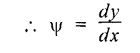
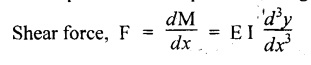
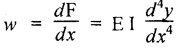
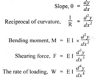
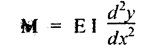
3. DIFFERENTIAL EQUATION OF DEFLECTED BEAM OR RELATION BETWEEN SLOPE, DEFLECTION AND RADIUS OF CURVATURE


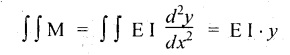
4. DOUBLE-INTEGRATION METHOD FOR SLOPE AND DEFLECTION


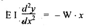
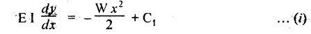
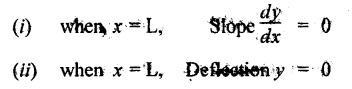
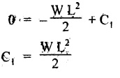
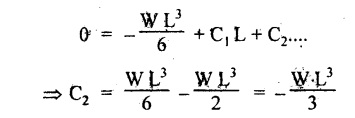
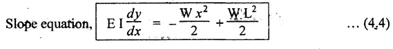
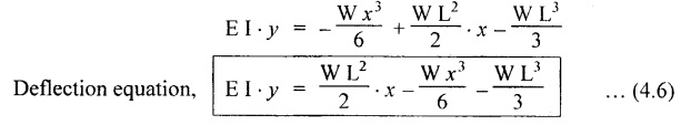
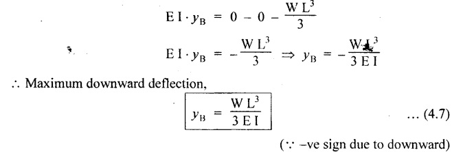
5. CANTILEVER WITH A POINT LOAD AT THE FREE END


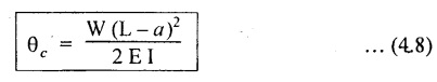
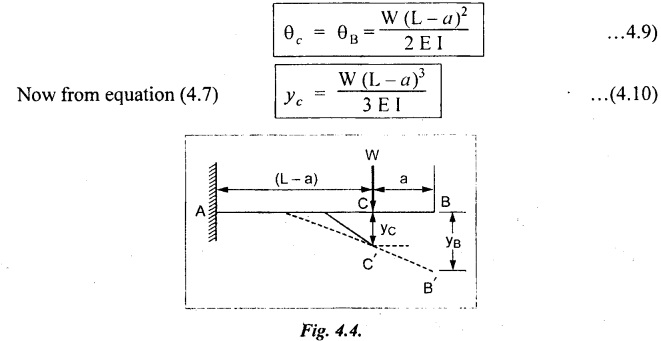
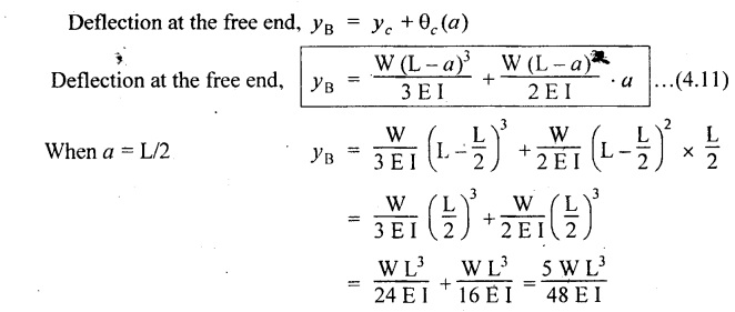
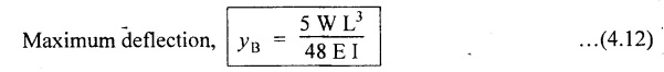
6. CANTILEVER WITH A POINT LOAD AT A DISTANCE OF 'a' FROM A FREE END
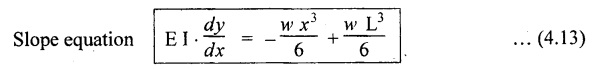
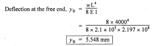
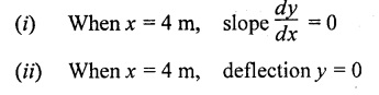
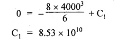
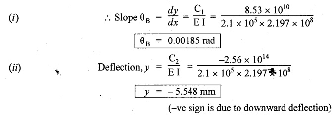
7. CANTILEVER WITH UDL


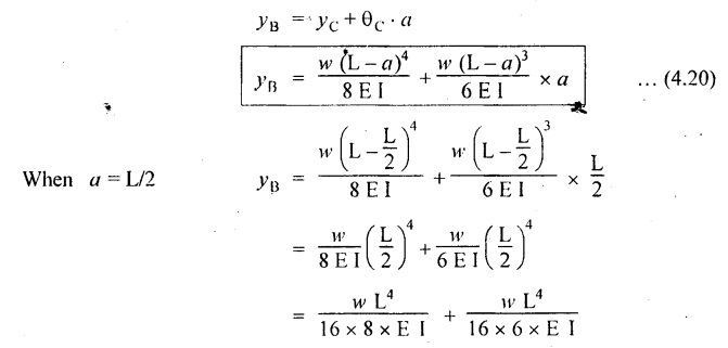
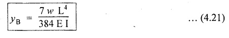
8. CANTILEVER WITH UDL FROM FIXED END


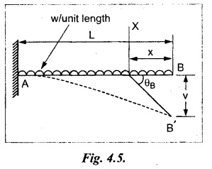
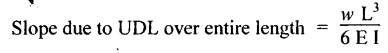
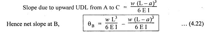
9. CANTILEVER WITH UDL FROM FREE END


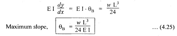
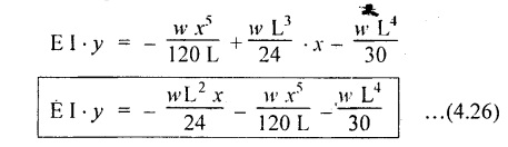
10. CANTILEVER WITH A UNIFORMLY VARYING LOAD (UVL)


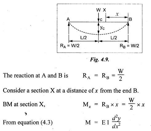
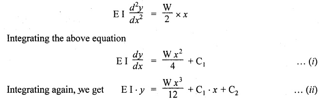
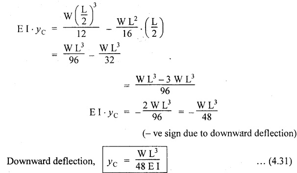
11. SIMPLY SUPPORTED BEAM (SSB) WITH CENTRAL POINT LOAD
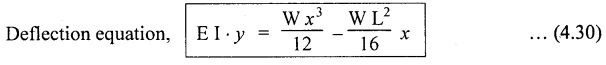
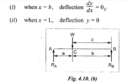
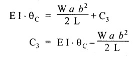
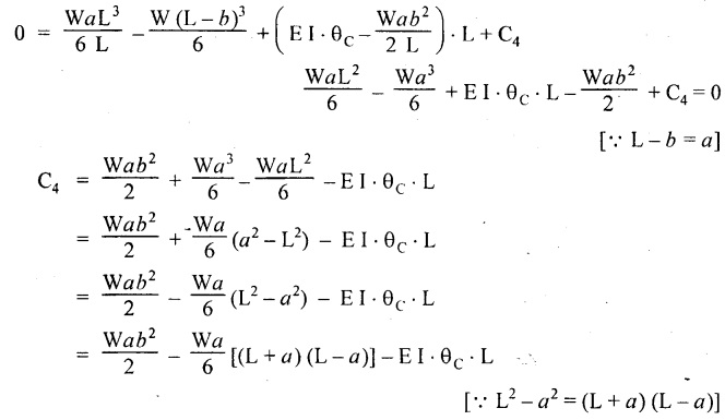
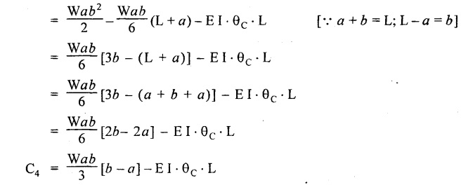
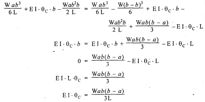
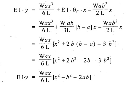
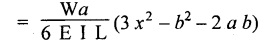
12. SSB WITH ECCENTRIC POINT LOAD


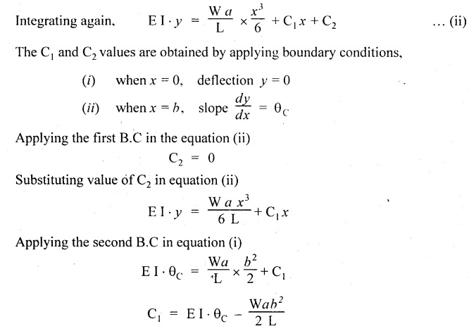
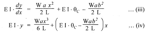
![]() is known.
is known.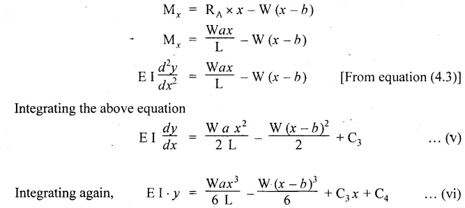

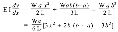
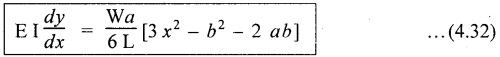


 Therefore, equating the slope equation (4.32) to zero.


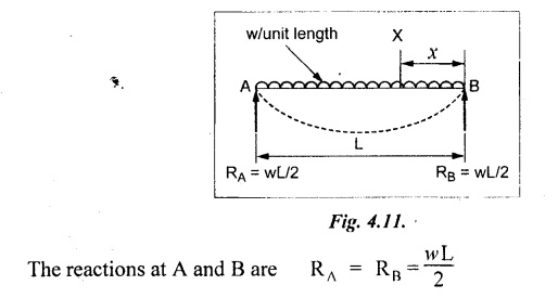
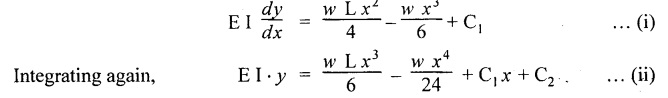
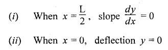
13. SSB WITH UDL


14. MACAULAY'S METHOD FOR SLOPE AND DEFLECTION

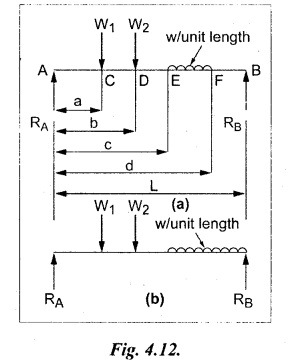


 Also n = 1 for a point load and n = 2 for UDL. This method is called Macaulay's method.

 (i.e., the term within brackets are to integrated as a whole). Similarly the quantity (x - b) should be integrated as a
  and so on.
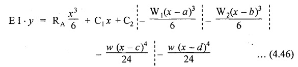
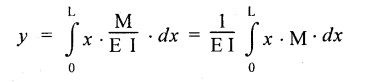
15. MOMENT AREA METHOD FOR SLOPE AND DEFLECTION


 is the area of B.M diagram between A and B.


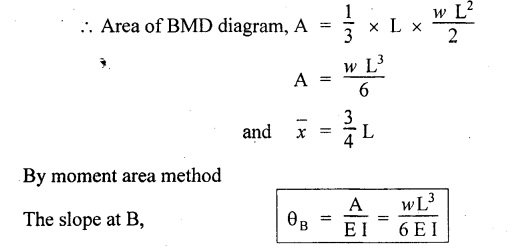
16. CANTILEVER WITH A POINT LOAD AT FREE END
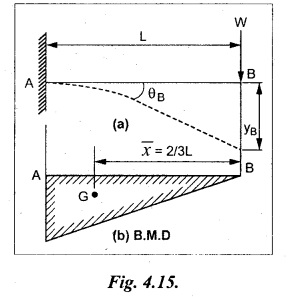


17. CANTILEVER WITH UDL


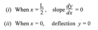
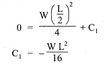
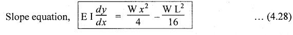
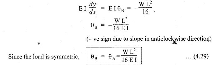
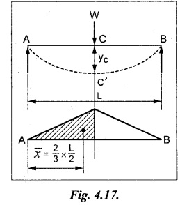
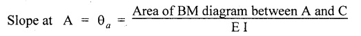
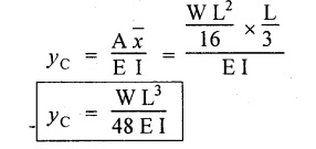
18. SSB WITH CENTRAL POINT LOAD

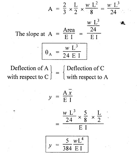
19. SSB WITH UDL

20. CONJUGATE BEAM METHOD
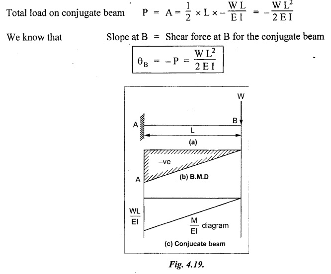
21. CANTILEVER WITH A POINT LOAD AT THE FREE END

22. CANTILEVER WITH UDL


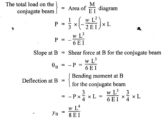
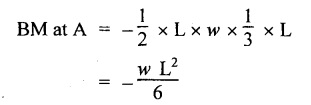
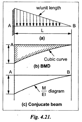
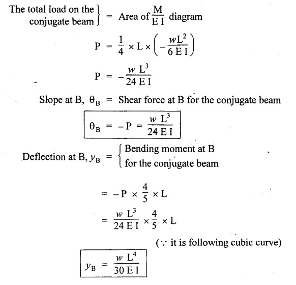
23. CANTILEVER WITH UNIFORMLY VARYING LOAD
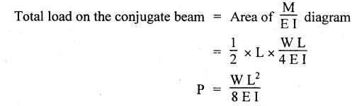
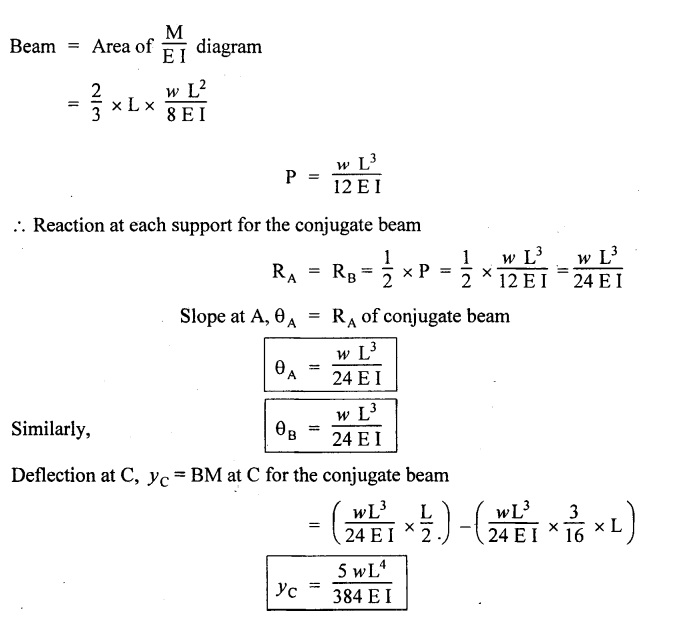
24. SSB WITH CENTRAL POINT LOAD


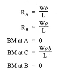
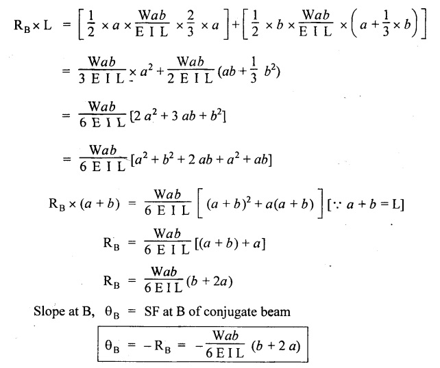
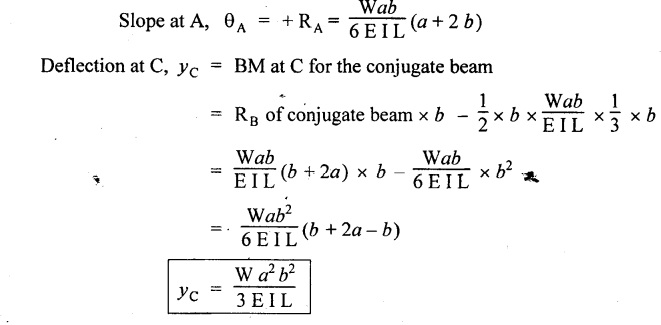
25. SSB WITH AN ECCENTRIC POINT LOAD


26. SSB WITH A UDL

![]() at the mid span of the beam 'C' parabolically.
at the mid span of the beam 'C' parabolically.![]()

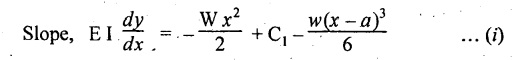
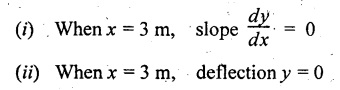
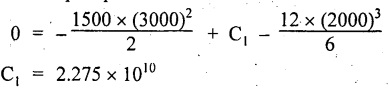
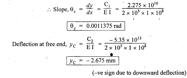
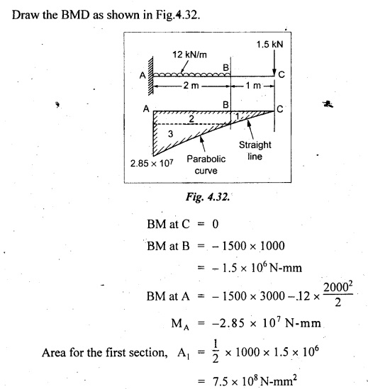
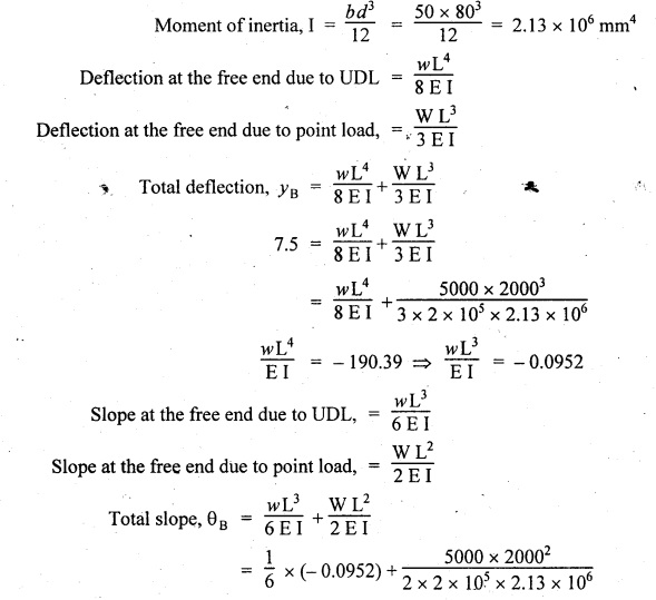
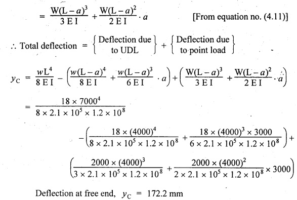
27. SOLVED PROBLEMS ON CANTILEVER BEAM


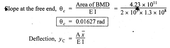

CONJUGATE BEAM METHOD


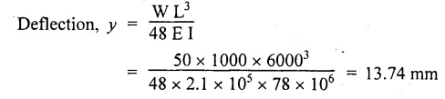
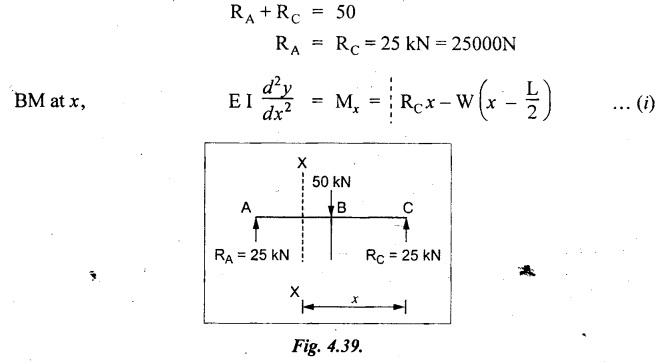
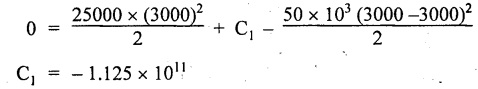
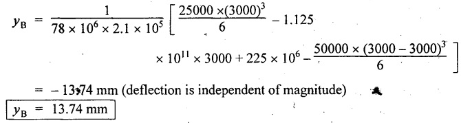
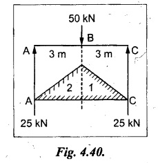
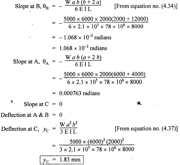
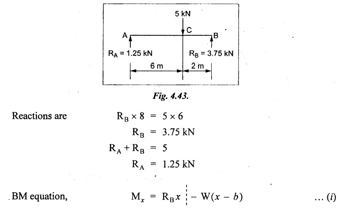
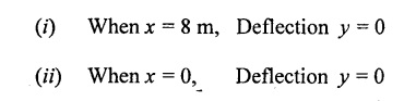
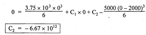
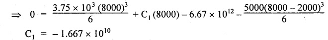
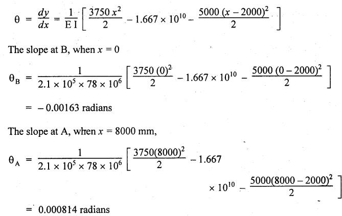
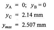
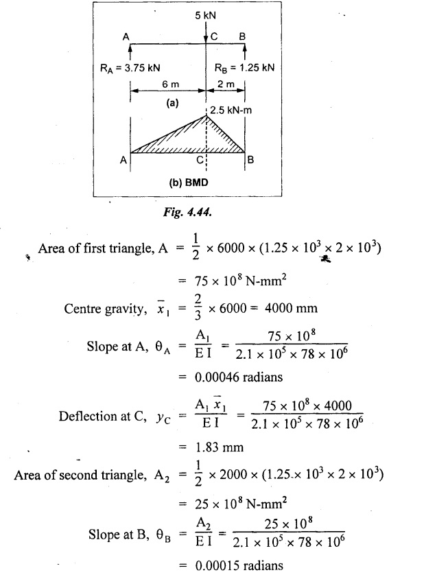
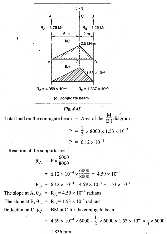
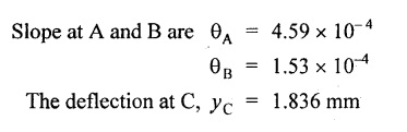
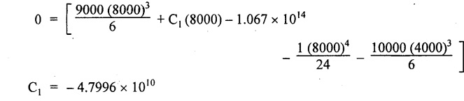
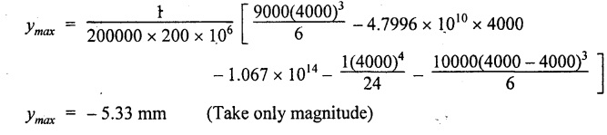
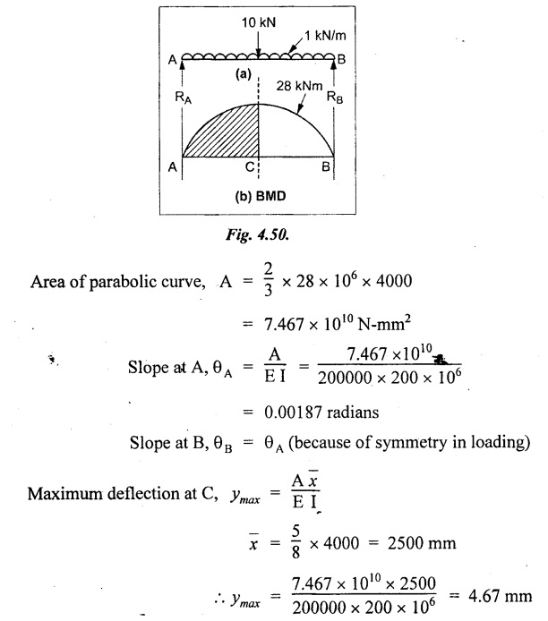
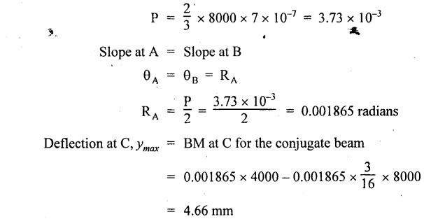
28. PROBLEMS ON SIMPLY SUPPORTED BEAM


29. STRAIN ENERGY AND DEFLECTION DUE TO BENDING UNDER GRADUALLY APPLIED LOADS


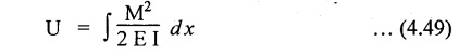

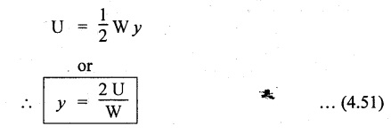
30. STRAIN ENERGY AND DEFLECTION DUE TO BENDING UNDER IMPACT LOADS


Strength of Materials: Unit IV: Deflection of Beams : Tag: : introduction - Deflection of Beams
Related Topics
Related Subjects
Strength of Materials
CE3491 4th semester Mechanical Dept | 2021 Regulation | 4th Semester Mechanical Dept 2021 Regulation