Theory of Machines: Unit I: Kinematics of Mechanisms
Acceleration in slider-crank mechanism
Kinematics of Mechanisms - Theory of Machines
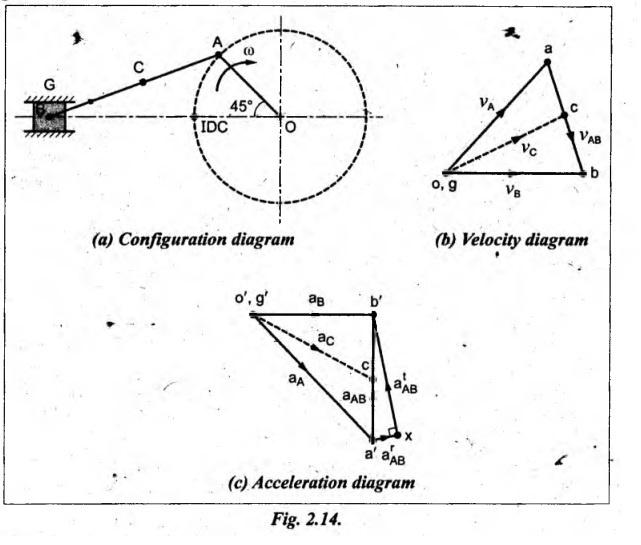
A slider-crank mechanism is shown in Fig.2.14(a). Crank OA rotates clockwise with uniform angular velocity ω rad/s.
ACCELERATION IN SLIDER-CRANK MECHANISM
A
slider-crank mechanism is shown in Fig.2.14(a). Crank OA rotates clockwise with
uniform angular velocity ω rad/s. It is required to draw the acceleration
diagram of the configuration.
Procedure:
Step 1: Configuration
diagram: First of all, draw the configuration
diagram, to some suitable scale, as shown in Fig.2.14(a).
Step 2: Velocity of
input link: When length of input link OA and its
angular velocity ωOA are known, then the velocity of input link (i.e.,
crank OA) is given by
vOA
= ωOA × OA (clockwise about O)
Step 3: Velocity
diagram: Now draw the velocity diagram, as
shown in Fig.2.14(b), to some suitable scale, using the procedure given
in Section 2.7.
Step 4: Velocity of
various links:
By
measurement from the velocity diagram, we get
Velocity
of the connecting rod, vBA = vector ab
and
Velocity of the slider, vBO = vector ob
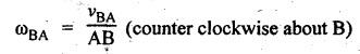
The
angular velocity of the connecting rod AB (ωBA) can be determined
using the relation
Step 5: Construction
of acceleration diagram:
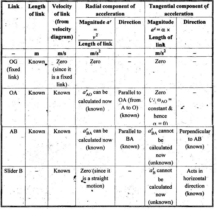
Using
the velocity of various links that are obtained with the help of velocity
diagram, the values of radial and tangential components of acceleration of
various link can be calculated "as shown in Table 2.3 below.
Table 2.3 Radial and tangential components of acceleration of
various links
Now
using the known values of magnitude and direction of acceleration components,
the acceleration diagram can be constructed, as shown in Fig.2.14(c), to
some suitable scale, using the procedure given below.
1.
Since the link AG is fixed, therefore take o' and g' as one
point.
2.
From point o', draw vector o'a' such that 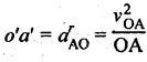 in the
direction parallel to OA to represent the radial component of acceleration of
link OA (i.e., arAO). Since atAO
= 0, therefore aAO = arAO.
in the
direction parallel to OA to represent the radial component of acceleration of
link OA (i.e., arAO). Since atAO
= 0, therefore aAO = arAO.
3.
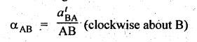
From point a', draw vector a'x such that a'x = arBA
= v2BA/AB in the direction parallel to BA to
represent the radial component of acceleration of link AB (i.e., arBA).
Now from point x, draw vector xb' perpendicular to AB to
represent the tangential component of acceleration of link AB (i.e., atBA)
whose magnitude is unknown.
4.
We know that the acceleration of slider B acts in the direction parallel to the
line of motion of slider B. So from point o', draw a vector o'b'
parallel to BO, intersecting the vector xb' at b'.
5.
Join points a' and b'.
Step 6: Acceleration
of various links:
Now
by measurement from the acceleration diagram, the various components of
acceleration of links can be found.
Acceleration
of slider, aBO = vector b'o'
Radial
component of acceleration of the connecting rod, arBA
= vector dx
Tangential
component of acceleration of the connecting rod, atBA
= vector b'x
Total
acceleration of the connecting rod, aBA = vector b'a'
Also
the angular acceleration of the connecting rod can be determined as
Example 2.6
ABCD is a four-bar chain with link AB fixed. The lengths of the
links are AB 62.5 mm; BC 175 mm; CD = 112.5 mm; and AD = 200 mm. The crank AB
rotates at 10 rad/s clockwise. Draw the velocity and acceleration diagram when
angle BAD 60° and B and C lie on the same side of AD. Find the angular velocity
and angular acceleration of links BC and CD.
[A.U.,
Nov/Dec 2011]
Given data:
AB
= 62.5 mm; BC = 175 mm; CD = 112.5 mm; AD = 200 mm; ωBA = 10 rad/s
(CW); ![]() BAD = 60°.
BAD = 60°.
Solution: Relative velocity
method.
Procedure:
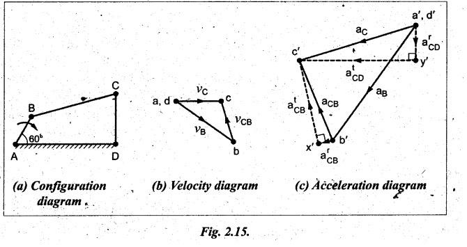
Step 1: Configuration
diagram: First of all, draw the configuration
diagram, to some suitable scale Gay, 1 cm = 40 mm), as shown in Fig.2.15(a).
Step 2: Velocity of
input link AB:
Velocity
of input link AB, vBA = ωBA × AB
=
10 × 0.0625 = 0.625 m/s
Step 3: Velocity
diagram: Now draw the velocity diagram, to
some suitable scale (say, 1 cm = 0.4 m/s), as shown in Fig.2.15(b),
using the procedure given in Example 2.1.
Step 4: Velocity of
various links:
By
measurement from the velocity diagram, we get
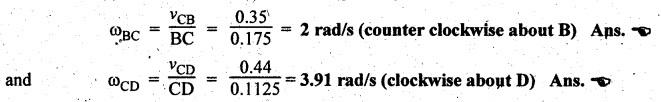
vCB
= vector bc = 0.35 m/s
and
vCD = vector dc = 0.44 m/s
The
angular velocity of links BC and CD are given by
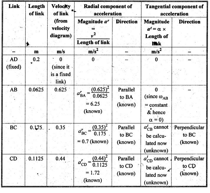
Step 5: Acceleration
diagram: The values of radial and tangential
components of acceleration of various links are calculated as shown in Table
2.4.
Table 2.4. Radial and tangential components of acceleration of
various links
Now
using the known values of magnitude and direction of acceleration components,
the acceleration diagram can be constructed, to some suitable. scale (say, 1 cm
= 1.5 m/s2), as shown in Fig.2.15(c), using the procedure
given in Section 2.11.
Step 6: Acceleration
of various links:
By
measurement from the acceleration diagram, we get
atCB
= vector xc' = 4.2 m/s2
atCD
= vector yc' = 5.5 m/s2
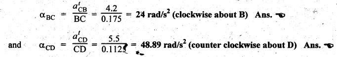
The
angular acceleration of links BC and CD are given by
Example 2.7
In a four-bar mechanism ABCD, the link lengths are as follows:
Input link AB = 25 mm; Coupler link BC = 85 mm; Output link CD = 50 mm; Frame
AD = 60 mm.
The angle between the frame and the input link is 100° measured
amiclockwise. The velocity of point B is 1.25 m/s in the clockwise direction.
(i) Sketch the mechanism.
(ii) Find the angular velocity and angular acceleration of links
BC and CD.
(iii) Determine the velocity and acceleration of the mid-point
of the link BC.
Given data:
AB
= 25 mm; BC = 85 mm; CD = 50 mm; AD = 60 mm; ![]() BAD = 100°; vB
= 1.25 m/s
BAD = 100°; vB
= 1.25 m/s
Solution: Relative velocity
method.
Procedure:
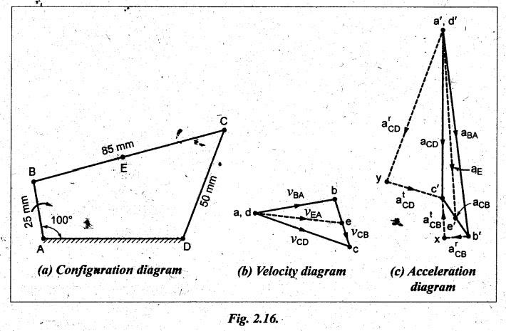
Step 1: Configuration
diagram: First of all, draw the configuration
diagram, to some suitable scale (say, 1 cm = 15 mm), as shown in Fig.2.16(a).
Step 2: Velocity of
input link AB:
Velocity
of input link AB, vBA = 1.25 m/s (clockwise) (given)
Step 3: Velocity
diagram: Now draw the velocity diagram, to
some suitable scale (say, 1 cm = 1 m/s), as shown in Fig.2.16(b), using
the procedure given in Example 2.1.
Note
In order to find the
velocity of mid-point E on link BC, divide the vector bc in the same ratio as E
divides BC. Since E is the mid-point of BC, therefore e is also mid-point of
vector bc.
Step 4: Velocity of
various links:
By
measurement from the velocity diagram, we get
Velocity
of link BC, vCB = vector
cb = 0.8 m/s
Velocity
of link CD, vCD = vector cd = 1.55 m/s
Velocity
of mid-point, E = vE = vector ed = 1.3 m/s Ans. ![]()
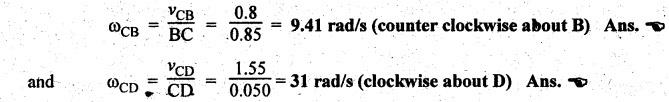
Angular
velocity of links BC and CD can be determined as
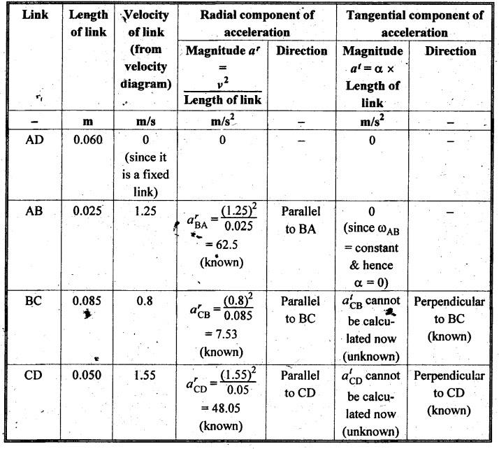
Step 5: Acceleration
diagram: The values of radial and tangential
components of acceleration of various links are calculated as shown in Table
2.5.
Table 2.5. Radial and tangential components of acceleration of
various links
Now
using the known values of magnitude and direction of acceleration components,
the acceleration diagram can be constructed, to some suitable scale (say, 1 cm
= 10 m/s2), as shown in Fig.2.16(c) using the procedure given in
Section 2.11.
Note
In order to find the acceleration of the
mid-point E on link BC, divide the vector b'c' in the same ratio as E
divides BC. Since E is the mid-point of BC, therefore e' is also
mid-point of vector b'c'.
Step 6: Acceleration
of various links:
By
measurement from the acceleration diagram, we get
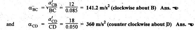
atCB
= vector xc' = 12 m/s2
atCD
= vector yc' = 18 m/s2
Acceleration
at mid-point E, aE = vector a'e' = 58 m/s2
Ans.
Now
the angular acceleration of links BC and CD are given by
Example 2.8
In a small steam engine running at 600 rad/min clockwise, length
of crank is 80 mm and•ratio of connecting rod length to crank radius is 3. For
the position when crank makes 45° to horizontal, determine:
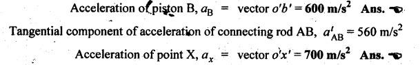
(i) the velocity and acceleration of the piston;
(ii) the angular velocity and angular acceleration of the
connecting rod; and
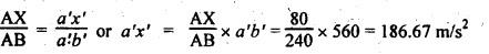
(iii) the linear velocity and acceleration of a point X on
connecting rod 80 mm from crank pin.
Given data:
ωOA
= 600 rad/min = 600/60 = 100 rad/s (CW); OA = 80 mm; n = l/r
= 3 or l = 3 r = 3 (80) = 240 mm; ![]() BOA = 45°
BOA = 45°
Solution: Relative velocity
method.
Procedure:
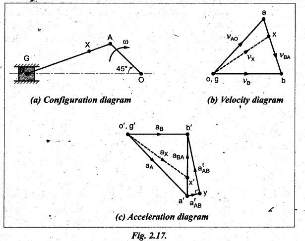
Step 1: Configuration
diagram: First of all, draw the configuration
diagram, to some suitable scale (say, 1 cm = 40 mm), as shown in Fig.2.17(a).
Step 2: Velocity of
input link:
Velocity
of crank OA is given by
vOA
= ωOA × OA = 100 × 0.080 = 8 m/s
Step 3: Velocity
diagram: Now draw the velocity diagram, as
shown in Fig.2.17(b), to some suitable scale (say, 1cm = 2 m/s), using the
procedure given in Section 2.7.
Step 4: Velocity of
various links:
By
measurement from the velocity diagram, we get
Velocity
of piston, vB = vector ab = 7 m/s Ans.
Velocity
of connecting rod, vBA = vector ab = 6 m/s
Velocity
of point X on AB, vX = vector x = 7 m/s Ans.
Note
In the velocity
diagram, the position of point x on the connecting rod can be obtained as
below.
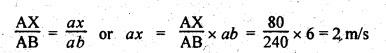
Now the angular
velocity of the connecting rod AB is given by

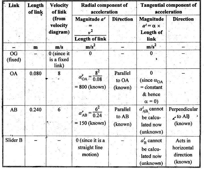
Step 5: Acceleration
diagram: The values of radial and tangential
components of acceleration of various links are calculated as shown in Table
2.6.
Table 2.5. Radial and tangential components of acceleration of
various links
Step 6: Acceleration
of various links:
By
measurement from the acceleration diagram, we get
Note
In the acceleration diagram, the position of
point x' on the connecting rod a'b' can be obtained as below.
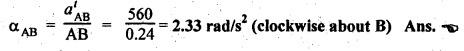
Now the angular
acceleration of the connection rod AB is given by
Example 2.9
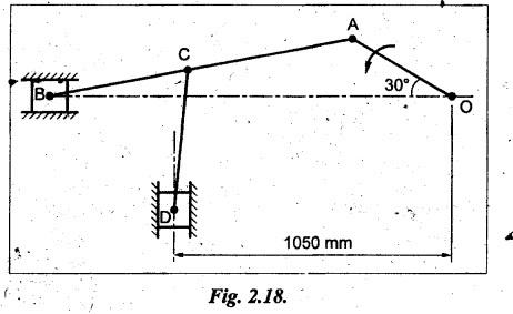
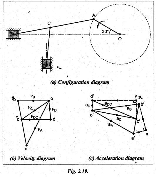
In the mechanism, as shown in Fig.2.18, the crank OA rotates at
20 rpm anticlockwise and gives motion to the sliding blocks B and D. The
dimensions of the various links are OA = 300 mm; AB = 1200 mm; BC≈ 450 mm and
CD = 450 mm.
For the given configuration, determine: (i) velocities of
sliding at B and D; (ii) angular velocity of CD; (iii) linear acceleration of
D; and (iv) angular acceleration of CD.
Given data:
NOA
= 20 rpm (CCW); OA = 300 mm; AB = 1200 mm; BC = 450 mm; CD = 450 mm
Solution: Relative velocity
method.
Procedure:
Step 1: Configuration
diagram: First of all, draw the configuration
diagram, to some suitable scale (say, 1 cm = 200 mm), as shown in Fig.2.19(a).
Step 2: Velocity of
input link:
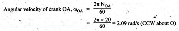
Velocity
of crank OA, vOA = ωAO × ΑΟ
=
2.09 × 0.3 = 0.627 m/s
Step 3: Velocity
diagram: Now draw the velocity diagram, to
some suitable scale (say, 1 cm = 0.2 m/s), as shown in Fig.2.19(b).
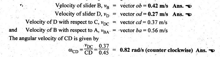
Step 4: Velocity of
various links:
By
measurement from the velocity diagram, we get
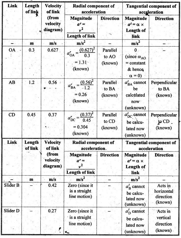
Step 5: Acceleration
diagram: The values of radial and tangential
components of acceleration of various links are calculated as shown in Table
2.7.
Table 2.7. Radial and tangential components of acceleration
Now
using the known values of magnitude and direction of acceleration components,
the acceleration diagram can be constructed, to some suitable scale (say, 1 cm
= 0.3 m/s2), as shown in Fig.2.19(c).
Step 6: Acceleration
of various links:
By
measurement from the acceleration diagram, we get
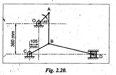
Example 2.10
In the toggle mechanism shown in Fig.2.20, the slider D is
constrained to move on a horizontal path. The crank OA is rotating in the
counter clockwise direction at a speed of 180 rpm increasing at the rate of 50
rad/s. The dimensions of the various links are as follows:
OA = 180 mm; CB = 240 mm; AB = 360 mm; and BD = 540 mm.
For the given configuration, determine:
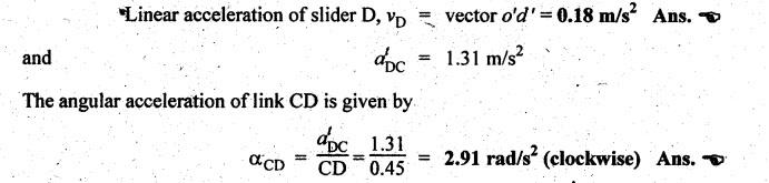
(i) the velocity of the slider D;
(ii) the angular velocity and angular acceleration of links AB,
BC and BD; and
(iii) the linear acceleration of the slider D.
Given data:
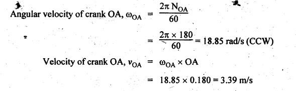
NOA
= 180 rpm (CCW); αOA = 50 rad/s2; OA = 180 mm; CB = 240
mm; AB = 360 mm; BD = 540 mm
Solution: Relative velocity
method.
Procedure:
Step 1: Configuration
diagram: First of all, draw the configuration
diagram, to some suitable scale (say, 1 cm = 20 mm), as shown in Fig.2.21(a).
Step 2: Velocity of
input link:
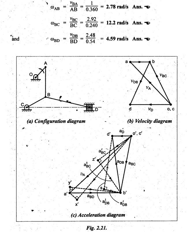
Step 3: Velocity
diagram: Now draw the velocity diagram, to
some suitable scale (say, 1 cm = 0.75 m/s), as shown in Fig.2.21(b).
Step 4: Velocity of
various links:
By
measurement from the velocity diagram, we get
vD
= vector cd = 2.12 m/s Ans.
vBA
= vector ab = 1 m/s
vBC
= vector cb = 2.92 m/s
vDB
= vector bd = 2.48 m/s
The
angular velocity of links AB, BC and BD are given by
Step 5: Acceleration
diagram: The value of radial and tangential
components of acceleration of various links are calculated as shown in Table
2,8.
Table 2.8. Radial and tangential components of acceleration
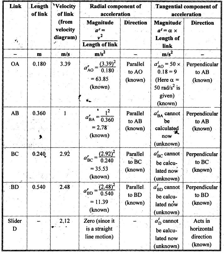
Now
using the known values of magnitude and direction of acceleration components,
the acceleration diagram can be constructed, to some suitable scale (say, 1 çm
10 m/s2), as shown in Fig.2.21(c).
Step 6: Acceleration
of various links:
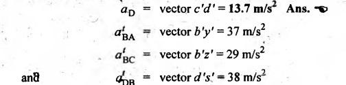
By
measurement from the acceleration diagram, we get
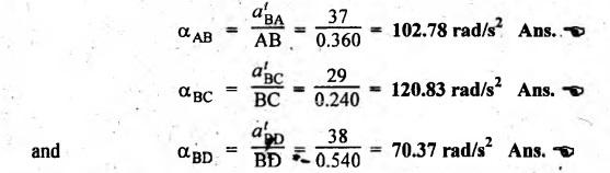
The
angular acceleration of links AB, BC and CD are given by
Theory of Machines: Unit I: Kinematics of Mechanisms : Tag: : Kinematics of Mechanisms - Theory of Machines - Acceleration in slider-crank mechanism
Related Topics
Related Subjects
Theory of Machines
ME3491 4th semester Mechanical Dept | 2021 Regulation | 4th Semester Mechanical Dept 2021 Regulation